Welcome to coolpup.py’s documentation!

Project homepage with code and issues is on GitHub.

Please feel free to report any problems or contribute.

coolpup.py

.cool file pile-ups with python.

A versatile tool to perform pile-up analysis on Hi-C data in .cool format (https://github.com/mirnylab/cooler). And who doesn’t like cool pupppies?

Introduction

What are pileups?

Pileups is the generic term we use to describe any procedure that averages multiple 2D regions (snippets) of a 2D matrix, e.g. Hi-C data. In some contexts they are also known as APA (aggregate peak analysis, from Rao et al., 2014), or aggregate region/TAD analysis (in GENOVA, van der Weide et al., 2021), and other names. The most typical use case is to quantify average strength of called dots (loops) in Hi-C data, or strength of TAD boundaries. However the approach can do much more than that. This is the idea of how pileups work to check whether certain regions tend to interact with each other:

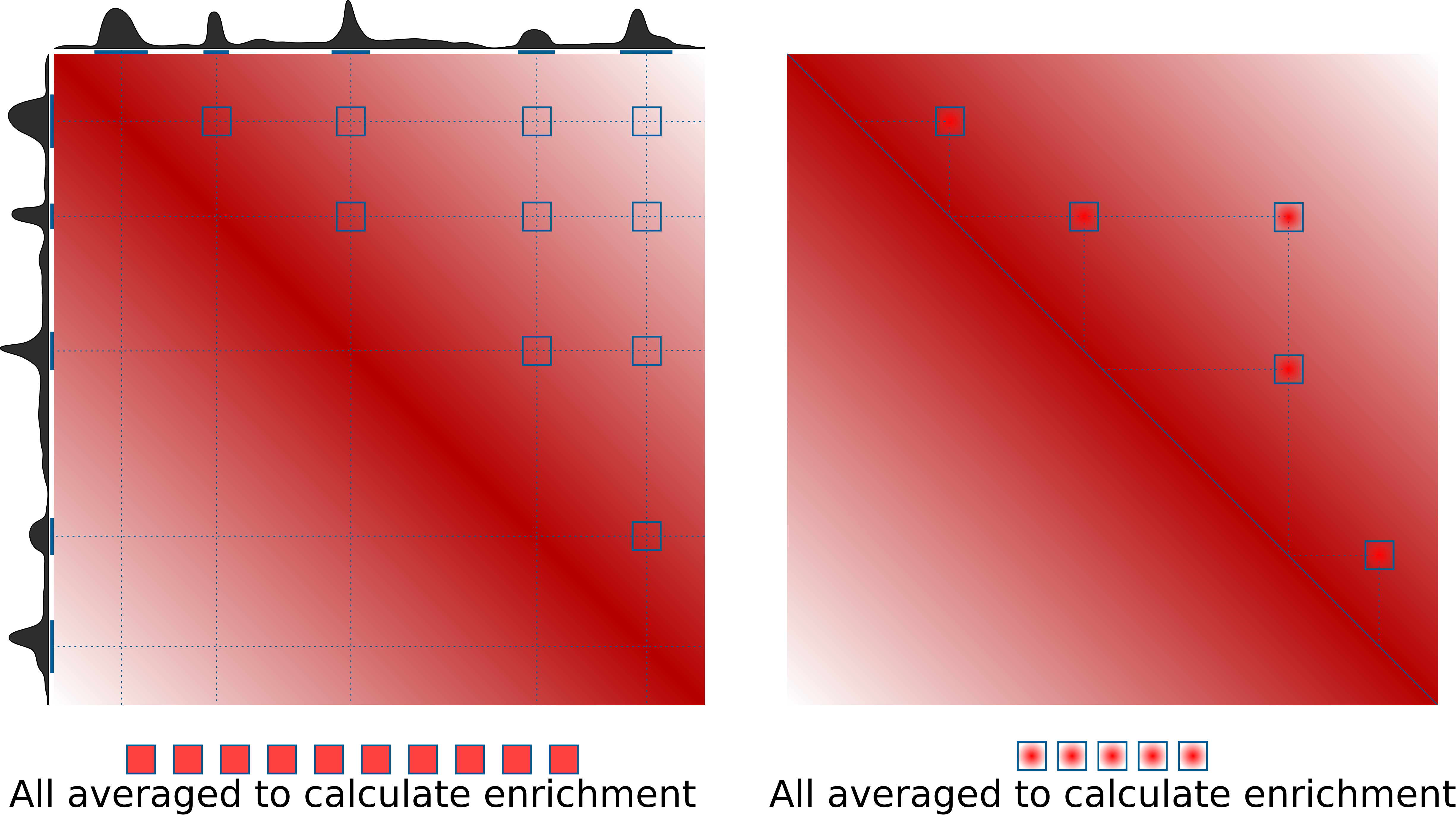
On the right is the more typical use case for quantification of loop strength. On the left is a different approach, designed to check whether specific regions in the genome (e.g. binding sites of a certain factor) tend to interact with each other.

What is very important for this quantification, is the normalization to expected values. This can be done in two ways: either using a chromosome- (or arm-) wide by-distance expected interactions, using a file with average values of interactions at different distances (e.g. output of cooltools expected-cis), or directly from Hi-C data by dividing the pileups over randomly shifted control regions. If neither expected normalization approach is used (just set --nshifts 0), this becomes essentially identical to the APA approach (Rao et al., 2014), which can be used for averaging strongly interacting regions, e.g. annotated loops. For weaker interactors, decay of contact probability with distance can hide any focal enrichment that could be observed otherwise. However, most importantly, when comparing different sets of regions at even slightly different distances, or comparing different datasets, the decay of contact probability with distance will very strongly affect the resulting values, hence normalizing to it is essential in many cases, and generally recommended.

coolpup.py vs cooltools pileup

cooltools is the main package with Hi-C analysis maintained by open2C. It also has a tool to perform pileups. Why does coolpup.py exit then? The way cooltools pileup works, is it accumulates all snippets for the pileup into one 3D array (stack). Which gives a lot of flexibility in case one wants to subset the snippets based on some features later, or do some other non-standard computations based on the stack. But this is only advantageous when one performs analysis using the Python API, and moreover limits the application of cooltools pileup so it can’t be applied to a truly large number of snippets due to memory requirements. That’s where coolpup.py comes in: internally it never stores more than one snippet in memory, hence there is no limit to how many snippets can be processed. coolpup.py is particularly well suited performance-wise for analysing huge numbers of potential interactions, since it loads whole chromosomes into memory one by one (or in parallel to speed it up) to extract small submatrices quickly. Having to read everything into memory makes it relatively slow for small numbers of loops, but performance doesn’t decrease until you reach a huge number of interactions. Additionally, cooltools pileup doesn’t support inter-chromosomal (trans) pileups, however it is possible in coolpup.py.

While there is no way to subset the snippets after the pileup is generated (since they are not stored), coolpup.py allows one to perform various subsetting during the pileup procedure. Builtin options in the CLI are subsetting by distance, by strand, by strand and distance at the same time, and by window/region - in case of a provided BED file, one pileup is generated for each row against all others in the same chromosome; in case of trans-pileups, pileups for each chromosome pair can be generated. Importantly, in Python API any arbitrary grouping of snippets is possible.

.cool format

.cool is a modern and flexible format to store Hi-C data. It uses HDF5 to store a sparse representation of the Hi-C data, which allows low memory requirements when dealing with high resolution datasets. Another popular format to store Hi-C data, .hic, can be converted into .cool files using hic2cool (https://github.com/4dn-dcic/hic2cool).

See for details:

Abdennur, N., and Mirny, L. (2019). Cooler: scalable storage for Hi-C data and other genomically-labeled arrays. Bioinformatics. 10.1093/bioinformatics/btz540

Getting started

Installation

All requirements apart are available from PyPI or conda.

Before installing everything you need to obtain Cython using either pip or conda. Then for coolpuppy (and other dependencies) simply do:

pip install coolpuppy

or

pip install https://github.com/open2c/coolpuppy/archive/master.zip

to get the latest version from GitHub. This will make coolpup.py callable in your terminal, and importable in python as coolpuppy.

Usage

The basic usage syntax is as follows:

coolpup.py [OPTIONS] coolfile.cool regionfile.bed

A guide walkthrough to pile-up analysis is available here (WIP): Walkthrough

Docs for the command line interface are available here: CLI docs

Some examples to get you started with CLI interface are available here and for the python API examples see here.

Plotting results

For flexible plotting, I suggest to use matplotlib or another library. However simple plotting capabilities are included in this package. Just run plotpup.py with desired options and list all the output files of coolpup.py you’d like to plot.

Citing coolpup.py

Ilya M Flyamer, Robert S Illingworth, Wendy A Bickmore (2020). Coolpup.py: versatile pile-up analysis of Hi-C data. Bioinformatics, 36, 10, 2980–2985.

https://academic.oup.com/bioinformatics/article/36/10/2980/5719023

doi: 10.1093/bioinformatics/btaa073

Guide to pileup analysis

Coolpup.py is a tool for pileup analysis. But what are pile-ups?

If you don’t know, you might have seen average ChIP-seq or ATAC-seq profiles which look something like this:

Pile-ups in Hi-C are essentially the same as average profiles, but in 2 dimensions, since Hi-C data is a a matrix, not a linear track!

Therefore instead of a linear plot, pileups are usually represented as heatmaps - by mapping values of different pixels in the average matrix to specific colours.

Pile-ups of interactions between a set of regions

For example, we can again start with ChIP-seq peaks, but instead of averaging ChIP-seq data around them, combine them with Hi-C data and check whether these regions are often found in proximity to each other. The algorithm is simple: we find intersections of all peaks in the Hi-C matrix (with some padding around the peak), and average them. If the peaks often interact, we will detect an enrichment in the centre of the average matrix:

Here is a real example:

Here I averaged all (intra-chromosomal) interactions between highly enriched ChIP-seq peaks of RING1B in mouse ES cells. I added 100 kbp padding to each bin containing the peak, and since I used 5 kbp resolution Hi-C data, the total length of each side of this heatmap is 205 kbp. I also normalizes the result by what we would expect to find by chance, and therefore the values indicate observed/expected enrichment. Because of that, the colour is log-scaled, so that the neutral grey colour corresponds to 1 - no enrichment or depletion, while red and blue correspond to value above and below 1, respectively.

What is important, is that in the center we see higher values than on the edges: this means that regions bound by RING1B tend to stick together more, than expected! The actual value in the central pixel is displayed on top left for reference.

This analysis is the default mode when coolpup.py is run with a .bed file, e.g. coolpup.py my_hic_data.cool my_protein_peaks.bed (with optional --expected my_hic_data_expected.tsv for normalization to the background level of interactions).

Pile-ups of predefined regions pairs, e.g. loops

A similar approach is based on averaging predefined 2D regions corresponding to interactions of specific pairs of regions. A typical example would be averaging loop annotations. This is very useful to quantify global perturbations of loop strength (e.g. annotate loops in WT, compare their strength in WT vs KO of an architectural protein), or to quantify them in data that are too sparse, such as single-cell Hi-C. The algorithm is very simple:

And here is a real example of CTCF-associated loops in ES cells:

Comparing with the previous example, you can clearly see that if you average loops that have been previously identified you, of course, get much higher enrichment of interactions, than if you are looking for a tendency of some regions to interact.

This analysis is performed with coolpup.py when instead of a bed file you provide a .bedpe file, so simply coolpup.py my_hic_data.cool my_loops.bedpe (with optional --expected my_hic_data_expected.tsv for normalization to the background level of interactions). bedpe is a simple tab-separated 6-column file with chrom1, start1, end1, chrom2, start2, end2.

Local pileups

A very similar approach can be used to quantify local properties in Hi-C maps, such as insulation. Valleys of insulation score can be identified (e.g. using cooltools diamond-insulation), or another way of identifying potential TAD boundaries can be used. Then regions around their positions can be averaged, and this can be used to visualize and quantify insulation in the same or another sample:

Here is an example of averaged insulation score valleys in mouse ES cells:

One can easily observe that these regions on average indeed have some insulating properties, and moreover the stripes emanating from the boundaries are very clear - they are a combination of real stripes found on edges of TADs in many cases, and loops found at different distances from the boundary in different TADs.

Average insulation can be quantiifed by dividing signal in two red squares (top left and bottom right corners) by the signal in the more blue squares (top right and bottom left corners), and here it is shown in the top left corner.

This analysis is very easily performed using coolpup.py: simply run coolpup.py my_hic_data.cool my_insulating_regions.bed --local (with optional --expected my_hic_data_expected.tsv for normalization to the background level of interactions; note that for local analyses in my experience random shift controls work better).

Rescaled pileups

If instead of boundary regions you have, for example, annotation of long domains, such as TADs, you can also average them to analyse internal interactions within these domains. The problem with simply applying the previous analysis to this case is that these domains can be of different length, and direct averaging will produce nonsensical results. However the submatrices corresponding to interactions within each domain (with some padding around) can all be individually rescaled to the same size, and then averaged. This way boundaries of these domains would be aligned in the final averaged matrices, and the pileups would make sense! here is a visual explanation of this idea:

And here is an example of such local rescaled pileups of TADs annotated using insulation score valleys used above in ES cells:

Each TAD was padded with the flanks of the same length as the TAD, and then they were all rescaled to 99x99 pixels. The pattern of the average TAD is very clear, in particular the corner loop at the top of the domain is highly enriched. Also the stripes, indicative of loop extrusion, both on the TAD borders and outside the TADs, are clearly visible.

You might notice that I removed the few central diagonals of the matrix here. That is because they are often noisy after this rescaling procedure, depending on the data you use.

To perform this analysis, you simply need to call coolpup.py my_hic_data.cool my_domains.bed --rescale --local (with optional --expected my_hic_data_expected.tsv for normalization to the background level of interactions). To specify the side of the final matrix as 99 bins add --rescale_size 99. Another useful option here is --rescale_pad, which defines the fraction of the original regions to use when padding them; the default value is 1, so each TAD is flanked on each side by a region of the same size.

Coolpuppy python API walkthrough notebook

Please see https://github.com/open2c/open2c_examples for detailed explanation of how snipping and pileups work, and explanation of some terminology

# If you are a developer, you may want to reload the packages on a fly. 
# Jupyter has a magic for this particular purpose:
%load_ext autoreload
%autoreload 2

# import standard python libraries
import matplotlib as mpl
%matplotlib inline
mpl.rcParams['figure.dpi'] = 96
import numpy as np
import matplotlib.pyplot as plt
import pandas as pd
import seaborn as sns

# import libraries for biological data analysis
from coolpuppy import coolpup
from coolpuppy.lib import numutils
from coolpuppy.lib.puputils import divide_pups
from coolpuppy import plotpup
import cooler
import bioframe
import cooltools
from cooltools import expected_cis, expected_trans
from cooltools.lib import plotting

Download data

For the test, we collected the data from immortalized human foreskin fibroblast cell line HFFc6:

• Micro-C data from Krietenstein et al. 2020

• ChIP-Seq for CTCF from ENCODE ENCSR000DWQ

You can automatically download test datasets with cooltools. More information on the files and how they were obtained is available from the datasets description.

# Print available datasets for download
cooltools.print_available_datasets()

1) HFF_MicroC : Micro-C data from HFF human cells for two chromosomes (hg38) in a multi-resolution mcool format. 
	Downloaded from https://osf.io/3h9js/download 
	Stored as test.mcool 
	Original md5sum: e4a0fc25c8dc3d38e9065fd74c565dd1

2) HFF_CTCF_fc : ChIP-Seq fold change over input with CTCF antibodies in HFF cells (hg38). Downloaded from ENCODE ENCSR000DWQ, ENCFF761RHS.bigWig file 
	Downloaded from https://osf.io/w92u3/download 
	Stored as test_CTCF.bigWig 
	Original md5sum: 62429de974b5b4a379578cc85adc65a3

3) HFF_CTCF_binding : Binding sites called from CTCF ChIP-Seq peaks for HFF cells (hg38). Peaks are from ENCODE ENCSR000DWQ, ENCFF498QCT.bed file. The motifs are called with gimmemotifs (options --nreport 1 --cutoff 0), with JASPAR pwm MA0139. 
	Downloaded from https://osf.io/c9pwe/download 
	Stored as test_CTCF.bed.gz 
	Original md5sum: 61ecfdfa821571a8e0ea362e8fd48f63

# Downloading test data for pileups
# cache = True will download the data only if it was not previously downloaded
# data_dir="./" will force download to the current directory
cool_file = cooltools.download_data("HFF_MicroC", cache=True, data_dir='./')
ctcf_peaks_file = cooltools.download_data("HFF_CTCF_binding", cache=True, data_dir='./')
ctcf_fc_file = cooltools.download_data("HFF_CTCF_fc", cache=True, data_dir='./')

resolution = 10000
# Open cool file with Micro-C data:
clr = cooler.Cooler(f'{cool_file}::/resolutions/{resolution}')

# Use bioframe to fetch the genomic features from the UCSC.
hg38_chromsizes = bioframe.fetch_chromsizes('hg38')
hg38_cens = bioframe.fetch_centromeres('hg38')
hg38_arms = bioframe.make_chromarms(hg38_chromsizes, hg38_cens)

# Select only chromosomes that are present in the cooler. 
# This step is typically not required! we call it only because the test data are reduced. 
hg38_arms = hg38_arms.set_index("chrom").loc[clr.chromnames].reset_index()
# call this to automaticly assign names to chromosomal arms:
hg38_arms = bioframe.make_viewframe(hg38_arms)

hg38_arms

	chrom	start	end	name
0	chr2	0	93139351	chr2_p
1	chr2	93139351	242193529	chr2_q
2	chr17	0	24714921	chr17_p
3	chr17	24714921	83257441	chr17_q

hg38_arms.to_csv('hg38_arms.bed', sep='\t', header=False, index=False) # To use in CLI

# Read CTCF peaks data and select only chromosomes present in cooler:
ctcf = bioframe.read_table(ctcf_peaks_file, schema='bed').query(f'chrom in {clr.chromnames}')
ctcf['mid'] = (ctcf.end+ctcf.start)//2
ctcf.head()

	chrom	start	end	name	score	strand	mid
17271	chr17	118485	118504	MA0139.1_CTCF_human	12.384042	-	118494
17272	chr17	144002	144021	MA0139.1_CTCF_human	11.542617	+	144011
17273	chr17	163676	163695	MA0139.1_CTCF_human	5.294219	-	163685
17274	chr17	164711	164730	MA0139.1_CTCF_human	11.889376	+	164720
17275	chr17	309416	309435	MA0139.1_CTCF_human	7.879575	-	309425

import bbi

# Get CTCF ChIP-Seq fold-change over input for genomic regions centered at the positions of the motifs

flank = 250 # Length of flank to one side from the boundary, in basepairs
ctcf_chip_signal = bbi.stackup(
    ctcf_fc_file, 
    ctcf.chrom, 
    ctcf.mid-flank, 
    ctcf.mid+flank, 
    bins=1)

ctcf['FC_score'] = ctcf_chip_signal

ctcf['quartile_score']    = pd.qcut(ctcf['score'], 4, labels=False) + 1
ctcf['quartile_FC_score'] = pd.qcut(ctcf['FC_score'], 4, labels=False) + 1
ctcf['peaks_importance'] = ctcf.apply(
    lambda x: 'Top by both scores' if x.quartile_score==4 and x.quartile_FC_score==4 else
                'Top by Motif score' if x.quartile_score==4 else
                'Top by FC score' if x.quartile_FC_score==4 else 'Ordinary peaks', axis=1
)

# Select the CTCF sites that are in top quartile by both the ChIP-Seq data and motif score

sites = ctcf[ctcf['peaks_importance']=='Top by both scores']\
    .sort_values('FC_score', ascending=False)\
    .reset_index(drop=True)
sites.tail()

	chrom	start	end	name	score	strand	mid	FC_score	quartile_score	quartile_FC_score	peaks_importance
659	chr17	8158938	8158957	MA0139.1_CTCF_human	13.276979	-	8158947	25.056849	4	4	Top by both scores
660	chr2	176127201	176127220	MA0139.1_CTCF_human	12.820343	+	176127210	25.027294	4	4	Top by both scores
661	chr17	38322364	38322383	MA0139.1_CTCF_human	13.534864	-	38322373	25.010430	4	4	Top by both scores
662	chr2	119265336	119265355	MA0139.1_CTCF_human	13.739862	-	119265345	24.980141	4	4	Top by both scores
663	chr2	118003514	118003533	MA0139.1_CTCF_human	12.646685	-	118003523	24.957502	4	4	Top by both scores

sites.to_csv('annotated_ctcf_sites.tsv', sep='\t', index=False, header=False) # Let's save to use in CLI

On-diagonal pileup

On-diagonal pileup is the simplest, you need the positions of features (middlepoints of CTCF motifs) and the size of flanks aroung each motif. Coolpuppy will aggregate all snippets around each motif with the specified normalization.

pup = coolpup.pileup(clr, sites, features_format='bed', view_df=hg38_arms, local=True,
                        flank=300_000, min_diag=0)

INFO:coolpuppy:('chr2_p', 'chr2_p'): 144
INFO:coolpuppy:('chr2_q', 'chr2_q'): 202
INFO:coolpuppy:('chr17_p', 'chr17_p'): 78
INFO:coolpuppy:('chr17_q', 'chr17_q'): 239
INFO:coolpuppy:Total number of piled up windows: 663

This is the general format of output of coolpuppy pileup functions: a pandas dataframe with columns “data” and “n” - “data” contains pileups as numpy arrays, and “n” - number of snippets used to generate this pileup.

Different kinds of pileups calculated in one run are stored as rows, and their groups are annotated in the columns preceding “data”. Since here we didn’t split the data into any groups, there is only one pileup with group “all”

Let’s visualize the average Hi-C map at all strong CTCF sites:

plt.imshow(
    np.log10(pup.loc[0, 'data']),
    vmax = -1,
    vmin = -3.0,
    cmap='fall',
    interpolation='none')

plt.colorbar(label = 'log10 mean ICed Hi-C')
ticks_pixels = np.linspace(0, flank*2//resolution,5)
ticks_kbp = ((ticks_pixels-ticks_pixels[-1]/2)*resolution//1000).astype(int)
plt.xticks(ticks_pixels, ticks_kbp)
plt.yticks(ticks_pixels, ticks_kbp)
plt.xlabel('relative position, kbp')
plt.ylabel('relative position, kbp')

plt.show()

By-strand pileups

Now, we know that orientation of the CTCF site is very important for the interactions it forms. Using coolpuppy, splitting regions by the strand is trivial, expecially using a convenience function:

pup = coolpup.pileup(clr, sites, features_format='bed', view_df=hg38_arms, local=True,
                        by_strand=True,
                        flank=300_000, min_diag=0)

INFO:coolpuppy:('chr2_p', 'chr2_p'): 144
INFO:coolpuppy:('chr2_q', 'chr2_q'): 202
INFO:coolpuppy:('chr17_p', 'chr17_p'): 78
INFO:coolpuppy:('chr17_q', 'chr17_q'): 239
INFO:coolpuppy:Total number of piled up windows: 663

pup

	orientation	strand2	strand1	data	n	num	clr	resolution	flank	rescale_flank	...	rescale_size	flip_negative_strand	ignore_diags	store_stripes	nproc	by_window	by_strand	by_distance	groupby	cooler
0	--	-	-	[[1.8388677780141118, 0.3035714543313729, 0.05...	326	[[307, 307, 307, 306, 306, 306, 306, 307, 307,...	/gpfs/igmmfs01/eddie/wendy-lab/elias/coolpuppy...	10000	300000	None	...	99	False	0	False	1	False	True	False	[]	test
1	++	+	+	[[1.8534148775587997, 0.2993882425820983, 0.05...	337	[[325, 324, 324, 322, 322, 320, 320, 321, 320,...	/gpfs/igmmfs01/eddie/wendy-lab/elias/coolpuppy...	10000	300000	None	...	99	False	0	False	1	False	True	False	[]	test
2	all	all	all	[[1.846348485849592, 0.30142349774378974, 0.05...	663	[[632.0, 631.0, 631.0, 628.0, 628.0, 626.0, 62...	/gpfs/igmmfs01/eddie/wendy-lab/elias/coolpuppy...	10000	300000	None	...	99	False	0	False	1	False	True	False	[]	test

3 rows × 38 columns

Now we can use a convenient seaborn-based function from the plotpup.py subpackage to create a grid of heatmaps based on by-row and/or by-column variable mapping. In this case, we just map two orientations of CTCF sites across columns.

sns.set_theme(font_scale=2, style="ticks")
plotpup.plot(pup,
             cols='orientation', col_order=['--', '++'],
             score=False, cmap='fall', scale='log', sym=False,
             vmin=0.001, vmax=0.1,
             height=5)

<seaborn.axisgrid.FacetGrid at 0x7f756cb1b5e0>

Pileups of observed over expected interactions

Sometimes you don’t want to include the distance decay P(s) in your pileups. For example, when you make comparison of pileups between experiments and they have different P(s). Even if these differences are slight, they might affect the pileup of raw ICed Hi-C interactions. Moreover, without controlling for it the range of values in the pileup is not very easy to guess before plotting.

In this case, the observed over expected pileup is your choice. To normalize your pileup to the background level of interactions, you can either, prior to running the pileup function, calculate expected interactions for each chromosome arms, or you can generate randomly shifted control regions for each snippet, and divide the final pileup by that control pileup.

Let’s first try the latter. This analysis is particulalry useful for single-cell Hi-C where the data might be too sparse to generate robust per-diagonal expected values.

pup = coolpup.pileup(clr, sites, features_format='bed', view_df=hg38_arms, local=True,
                        by_strand=True, nshifts=10,
                        flank=300_000, min_diag=0)

INFO:coolpuppy:('chr2_p', 'chr2_p'): 144
INFO:coolpuppy:('chr2_q', 'chr2_q'): 202
INFO:coolpuppy:('chr17_p', 'chr17_p'): 78
INFO:coolpuppy:('chr17_q', 'chr17_q'): 239
INFO:coolpuppy:Total number of piled up windows: 663

plotpup.plot(pup,
             cols='orientation', col_order=['--', '++'],
             score=False, cmap='coolwarm', scale='log', sym=True,
             vmax=2,
             height=5)

<seaborn.axisgrid.FacetGrid at 0x7f756ca16cd0>

As you can see, this strongly highlights the depletion of interactions across the CTCF sites, and enrichment of interactions in a stripe starting from the site.

Now let’s calculate per-diagonal expected level of interactions to repeat the analysis using that.

# Calculate expected interactions for chromosome arms
expected = expected_cis(
    clr,
    ignore_diags=0,
    view_df=hg38_arms,
    chunksize=1000000)
expected.to_csv('test_expected_cis.tsv', sep='\t', index=False, header=True) # Let's save to use in CLI

pup = coolpup.pileup(clr, sites, features_format='bed', view_df=hg38_arms, local=True,
                        expected_df=expected, by_strand=True,
                        flank=300_000, min_diag=0)

INFO:coolpuppy:('chr2_p', 'chr2_p'): 144
INFO:coolpuppy:('chr2_q', 'chr2_q'): 202
INFO:coolpuppy:('chr17_p', 'chr17_p'): 78
INFO:coolpuppy:('chr17_q', 'chr17_q'): 239
INFO:coolpuppy:Total number of piled up windows: 663

plotpup.plot(pup,
             cols='orientation', col_order=['--', '++'],
             score=False, cmap='coolwarm', scale='log',
             sym=True, vmax=2,
             height=5)

<seaborn.axisgrid.FacetGrid at 0x7f756c9d5910>

The result is almost identical!

Instead of splitting two strands into two separate pileups, one can also flip the features on the negative strand. This way a single pileup is created where all features face in the same direction (as if they were on the positive strand). We can also add plot_ticks=True to show the central and flanking coordinates on the bottom of the plot.

pup = coolpup.pileup(clr, sites, features_format='bed', view_df=hg38_arms, local=True,
                        expected_df=expected, flip_negative_strand=True,
                        flank=300_000, min_diag=0)

INFO:coolpuppy:('chr2_p', 'chr2_p'): 144
INFO:coolpuppy:('chr2_q', 'chr2_q'): 202
INFO:coolpuppy:('chr17_p', 'chr17_p'): 78
INFO:coolpuppy:('chr17_q', 'chr17_q'): 239
INFO:coolpuppy:Total number of piled up windows: 663

plotpup.plot(pup,
             score=False, cmap='coolwarm', scale='log',
             sym=True, vmax=2,
             height=5, plot_ticks=True)

<seaborn.axisgrid.FacetGrid at 0x7f754d8d11f0>

Arbitrary grouping of snippets for pileups

Now, let’s see how our selection of only top CTCF peaks affects the results. We could simply repeat the analysis with the rest of CTCF peaks, but to showcase the power of coolpuppy, we’ll demonstrate how it can be used to generate pileups split be arbitrary categories

pup = coolpup.pileup(clr, ctcf, features_format='bed', view_df=hg38_arms, local=True,
                        expected_df=expected, flip_negative_strand=True,
                        groupby=['peaks_importance1'],
                        flank=300_000, min_diag=0)
# Splitting all snippets into groups based on annotated previously importance of the peaks
# Also flipping negative stranded features as shown above.

INFO:coolpuppy:('chr2_p', 'chr2_p'): 1381
INFO:coolpuppy:('chr2_q', 'chr2_q'): 2221
INFO:coolpuppy:('chr17_p', 'chr17_p'): 548
INFO:coolpuppy:('chr17_q', 'chr17_q'): 1602
INFO:coolpuppy:Total number of piled up windows: 5752

pup

	peaks_importance1	data	n	num	clr	resolution	flank	rescale_flank	chroms	minshift	...	rescale_size	flip_negative_strand	ignore_diags	store_stripes	nproc	by_window	by_strand	by_distance	groupby	cooler
0	Ordinary peaks	[[1.0699452226771298, 1.0642211188669746, 1.07...	3536	[[3432, 3421, 3412, 3413, 3403, 3404, 3402, 33...	/gpfs/igmmfs01/eddie/wendy-lab/elias/coolpuppy...	10000	300000	None	['chr2', 'chr17']	100000	...	99	True	0	False	1	False	False	False	[peaks_importance1]	test
1	Top by FC score	[[1.0829924317033595, 1.1009490059442415, 1.09...	778	[[745, 740, 741, 739, 739, 737, 739, 736, 734,...	/gpfs/igmmfs01/eddie/wendy-lab/elias/coolpuppy...	10000	300000	None	['chr2', 'chr17']	100000	...	99	True	0	False	1	False	False	False	[peaks_importance1]	test
2	Top by Motif score	[[1.0288083600349012, 1.0363397675639456, 1.03...	775	[[750, 749, 746, 744, 746, 741, 743, 743, 739,...	/gpfs/igmmfs01/eddie/wendy-lab/elias/coolpuppy...	10000	300000	None	['chr2', 'chr17']	100000	...	99	True	0	False	1	False	False	False	[peaks_importance1]	test
3	Top by both scores	[[1.0773804769093807, 1.0932965447911036, 1.09...	663	[[640, 638, 638, 635, 634, 632, 631, 630, 629,...	/gpfs/igmmfs01/eddie/wendy-lab/elias/coolpuppy...	10000	300000	None	['chr2', 'chr17']	100000	...	99	True	0	False	1	False	False	False	[peaks_importance1]	test
4	all	[[1.067003977204076, 1.0686994220484458, 1.072...	5752	[[5567.0, 5548.0, 5537.0, 5531.0, 5522.0, 5514...	/gpfs/igmmfs01/eddie/wendy-lab/elias/coolpuppy...	10000	300000	None	['chr2', 'chr17']	100000	...	99	True	0	False	1	False	False	False	[peaks_importance1]	test

5 rows × 36 columns

fg = plotpup.plot(pup.reset_index(), # Simply resetting the idnex makes the output directly compatible with the plotting function - 
                                                        # just need to remember there is also a group "all" which you might not want to show
                  cols='peaks_importance1',
                  col_order=['Ordinary peaks', 'Top by Motif score',
                             'Top by FC score', 'Top by both scores'],
                  score=False, cmap='coolwarm',
                  scale='log', sym=True, vmax=2,
                  height=5)

By-distance pileups

As it is known, CTCF sites frequently have peaks of Hi-C interactions between them, that indicate chromatin loops. Let’s see at what distances they tend to occur, and let’s see what patterns these regions form at different distance separations and different motif orientations.

Since we generate many more snippets than for local (on-diagonal) pileups, it will take a little longer to run. We can use the nproc argument to use multiprocessing and run it in parallel to speed it up a bit. Note that parallelization requires more RAM, so use with caution.

# Using all strong sites here to make it faster
pup = coolpup.pileup(clr, sites, features_format='bed', view_df=hg38_arms,
                        expected_df=expected, flip_negative_strand=True,
                        by_distance=True, by_strand=True, mindist=100_000,
                        flank=300_000, min_diag=0,
                        nproc=2
                        )
# Splitting all snippets into groups based on strand and separation between two sites

INFO:coolpuppy:('chr2_p', 'chr2_p'): 10250
INFO:coolpuppy:('chr17_p', 'chr17_p'): 2959
INFO:coolpuppy:('chr2_q', 'chr2_q'): 20215
INFO:coolpuppy:('chr17_q', 'chr17_q'): 28284
INFO:coolpuppy:Total number of piled up windows: 61708

pup.head()

	separation	orientation	distance_band	strand2	strand1	data	n	num	clr	resolution	...	rescale_size	flip_negative_strand	ignore_diags	store_stripes	nproc	by_window	by_strand	by_distance	groupby	cooler
0	0.1Mb-\n0.2Mb	++	(100000, 200000)	+	+	[[1.0169219164613472, 0.9600852237815437, 1.01...	67	[[64, 66, 66, 65, 66, 65, 63, 65, 65, 65, 65, ...	/gpfs/igmmfs01/eddie/wendy-lab/elias/coolpuppy...	10000	...	99	True	0	False	2	False	True	True	[]	test
1	0.2Mb-\n0.4Mb	++	(200000, 400000)	+	+	[[0.8621663934782983, 0.8441139544987121, 0.85...	131	[[125, 126, 126, 126, 126, 126, 125, 126, 126,...	/gpfs/igmmfs01/eddie/wendy-lab/elias/coolpuppy...	10000	...	99	True	0	False	2	False	True	True	[]	test
2	0.4Mb-\n0.8Mb	++	(400000, 800000)	+	+	[[0.6943248290614478, 0.6951043361705603, 0.68...	245	[[236, 236, 236, 236, 236, 236, 236, 236, 236,...	/gpfs/igmmfs01/eddie/wendy-lab/elias/coolpuppy...	10000	...	99	True	0	False	2	False	True	True	[]	test
3	0.8Mb-\n1.6Mb	++	(800000, 1600000)	+	+	[[0.6474314279066417, 0.6349530137034375, 0.68...	425	[[390, 390, 390, 390, 394, 389, 389, 393, 393,...	/gpfs/igmmfs01/eddie/wendy-lab/elias/coolpuppy...	10000	...	99	True	0	False	2	False	True	True	[]	test
4	1.6Mb-\n3.2Mb	++	(1600000, 3200000)	+	+	[[0.8110724673135341, 0.8450568161843092, 0.79...	789	[[727, 727, 727, 727, 732, 727, 718, 736, 734,...	/gpfs/igmmfs01/eddie/wendy-lab/elias/coolpuppy...	10000	...	99	True	0	False	2	False	True	True	[]	test

5 rows × 40 columns

fg = plotpup.plot(pup, rows='orientation', cols='separation',
                  row_order=['-+', '--', '++', '+-'],
                  score=False, cmap='coolwarm', scale='log', sym=True, vmax=3,
                  height=3)

Note that since CTCF sites are preferentially found in the A compartment, the expected level of interactions at different distances varies, generating different background interaction levels. We can artificially fix that by normalizing each pileup by the average interactions in the top-left and bottom-right corners.

fg = plotpup.plot(pup, rows='orientation', cols='separation',
                  row_order=['-+', '--', '++', '+-'],
                  score=False, cmap='coolwarm', scale='log', sym=True, vmax=3,
                  norm_corners=10,
                  height=3)

If you want to actually modify the data in your dataframe to normalize to the corners and not just apply it for vizualisation, you can do that explicitly:

pup['data'] = pup['data'].apply(numutils.norm_cis, i=10)

A good idea to give some more quantitative information about the level of enrichment of interactions in the center of the pileup is to just label the average value of the few central pixels of the heatmap. The simplest way is to use the argument score:

fg = plotpup.plot(pup, rows='orientation', cols='separation',
                  row_order=['-+', '--', '++', '+-'],
                  score=True,
                  cmap='coolwarm', scale='log', sym=True, vmax=3,
                  height=3)

Dividing pileups

Sometimes you may want to compare two pileups directly and plot the result of the division between them. For this we can use the divide_pups function. Let’s look at all CTCF interactions between 100 kb and 1 Mb by motif orientation.

pup = coolpup.pileup(clr, sites, features_format='bed', view_df=hg38_arms,
                        expected_df=expected,
                        by_strand=True, mindist=100_000, maxdist=1_000_000,
                        flank=300_000, nproc=2)

INFO:coolpuppy:('chr2_p', 'chr2_p'): 287
INFO:coolpuppy:('chr2_q', 'chr2_q'): 522
INFO:coolpuppy:('chr17_p', 'chr17_p'): 262
INFO:coolpuppy:('chr17_q', 'chr17_q'): 1235
INFO:coolpuppy:Total number of piled up windows: 2306

plotpup.plot(pup,
             cols="orientation",
             col_order=["-+", "--", "++", "+-"],
             score=False, cmap='coolwarm', scale='log',
             sym=True, vmax=2,
             height=2)

<seaborn.axisgrid.FacetGrid at 0x7f7631b5a850>

Let’s compare the ++ to the – CTCF motif orientation pileups. First, we have to create two separate pileup dataframes from the strand-separated pileups. Alternatively, you could generate two new pileups and store them. Importantly, the two pileups cannot differ with regards to the columns they contain and the resolution, flank size etc. they’ve been generated using.

pup_plus = pup.loc[pup["orientation"]=="++"].drop(columns=["strand1", "strand2", "orientation"])
pup_minus = pup.loc[pup["orientation"]=="--"].drop(columns=["strand1", "strand2", "orientation"])

pup_divide = divide_pups(pup_plus, pup_minus)

plotpup.plot(pup_divide,
                          score=False, cmap='PuOr_r', scale='log',
                          sym=True, height=4)

<seaborn.axisgrid.FacetGrid at 0x7f7631cebe50>

Stripe stackups

Oftentimes, as seen in the examples above, the interactions between regions are not just focal, but seen as stripes with enrichment along the vertical/horizontal axis from one or both of the anchor points. In the CTCF pileups from above we see a very strong corner stripe between +- sites, so let’s try to plot these individual stripes. Below is a schematic of what is meant by the different types of stripes.

We first have store this information when generating the pileup using the store_stripes=True argument which will add the columns vertical_stripe, and horizontal_stripe to the output. These are used to calculate the corner stripe in the plotting function.

pup = coolpup.pileup(clr, sites, features_format='bed', view_df=hg38_arms,
                        expected_df=expected,
                        by_strand=True, mindist=100_000, maxdist=1_000_000,
                        flank=300_000, nproc=2,
                        store_stripes=True)

INFO:coolpuppy:('chr2_p', 'chr2_p'): 287
INFO:coolpuppy:('chr2_q', 'chr2_q'): 522
INFO:coolpuppy:('chr17_p', 'chr17_p'): 262
INFO:coolpuppy:('chr17_q', 'chr17_q'): 1235
INFO:coolpuppy:Total number of piled up windows: 2306

We can plot the stripes using the the plot_stripes function

sns.set(font_scale = 1.3, style="ticks")
plotpup.plot_stripes(pup.loc[(pup["strand1"] == "+") &
                             (pup["strand2"] == "-"),:],
                     vmax=10, height=4, 
                     stripe="vertical_stripe", stripe_sort="sum",
                     plot_ticks=True)

<seaborn.axisgrid.FacetGrid at 0x7f76319c6b20>

Each line of the above plot represents the “corner stripe” between two regions. These pairs are sorted by the sum of the stripe by default, but we can also sort them by the central pixel, i.e. the pixel where the two regions of interest interact, with the stripe_sort argument. We can further save the pairs in the sorted order using out_sorted_bedpe. This file can then be used to inspect individual pairs with high contact frequencies. We can also add a lineplot with the average signal above the stripes using lineplot (note that this only works for single stripe plots.)

plotpup.plot_stripes(pup.loc[(pup["strand1"] == "+") &
                             (pup["strand2"] == "-"),:],
                     vmax=10, height=4, 
                     stripe="corner_stripe", plot_ticks=True,
                     stripe_sort="center_pixel", 
                     out_sorted_bedpe="CTCF_+-_sorted_centerpixel.bedpe",
                     lineplot=True)

<seaborn.axisgrid.FacetGrid at 0x7f754dc03cd0>

Rescaling

Pileups can also be rescaled to visualise enrichment within regions of interests of different sizes using rescale=True. The rescale_flank value represents how large the flanks are compared to the region of interest, where 1 is equal in size and for example 3 will be three times the size. The number of pixels in the final plot after rescaling is set with rescale_size. Let’s try this for B compartment interactions.

# Load cooler at 1 Mb resolution
clr_1Mb = cooler.Cooler(f'{cool_file}::/resolutions/1000000')
# Calculate eigenvectors
cis_eigs = cooltools.eigs_cis(clr_1Mb, n_eigs=3)
eigenvector_track = cis_eigs[1][['chrom','start','end','E1']]
# Extract B compartments
B_compartments = bioframe.merge(eigenvector_track[eigenvector_track["E1"] < 0], min_dist=0)
# Let's save to use it in CLI
B_compartments[["chrom", "start", "end"]].to_csv("B_compartments.bed", sep="\t", header=None, index=False)

pup = coolpup.pileup(clr, B_compartments, features_format='bed', view_df=hg38_arms,
                        expected_df=expected,
                        rescale=True, rescale_flank=1, rescale_size=99,
                        flank=300_000, nproc=2)

INFO:coolpuppy:Rescaling with rescale_flank = 1 to 99x99 pixels
INFO:coolpuppy:('chr2_p', 'chr2_p'): 36
INFO:coolpuppy:('chr17_p', 'chr17_p'): 6
INFO:coolpuppy:('chr17_q', 'chr17_q'): 21
INFO:coolpuppy:('chr2_q', 'chr2_q'): 153
INFO:coolpuppy:Total number of piled up windows: 216

fg = plotpup.plot(pup,
                  score=False, cmap='coolwarm', scale='log', 
                  sym=True, vmax=2, height=3)

Trans (inter-chromosomal) pileups

We can also perform pileups between regions on different chromosomes. We will try this for insulation score boundaries (TAD boundaries), first for cis (within chromosomes) and then for trans (between chromosomes).

# Call insulation score at windows of 50 kb
insulation_table = cooltools.insulation(clr, [50000], verbose=True)
# Select strong boundaries
strong_boundaries = insulation_table.loc[insulation_table["boundary_strength_50000"] > 1.5, :]
# Let's save to use it in CLI
strong_boundaries[["chrom", "start", "end"]].to_csv("strong_boundaries.bed", sep="\t", header=None, index=False)

INFO:root:Processing region chr2
INFO:root:Processing region chr17

pup = coolpup.pileup(clr, strong_boundaries, features_format='bed', view_df=hg38_arms,
                        expected_df=expected,
                        flank=300_000, nproc=2)

INFO:coolpuppy:('chr2_p', 'chr2_p'): 807
INFO:coolpuppy:('chr17_p', 'chr17_p'): 99
INFO:coolpuppy:('chr2_q', 'chr2_q'): 2262
INFO:coolpuppy:('chr17_q', 'chr17_q'): 1354
INFO:coolpuppy:Total number of piled up windows: 4522

plotpup.plot(pup,
             score=False, cmap='coolwarm', scale='log',
             sym=True, vmax=2,
             height=3)

<seaborn.axisgrid.FacetGrid at 0x7f763151f8e0>

Here we can see the boundary pileups within chromosome arms where interactions are depleted at the boundaries. To perform the same analysis between chromosomes, we first need to generate a new expected file (or use shifted controls) and then run the analysis with trans=True.

# Calculate expected interactions between chromosomes
trans_expected = expected_trans(
    clr, 
    chunksize=1000000)

trans_expected

	region1	region2	n_valid	count.sum	balanced.sum	count.avg	balanced.avg
0	chr2	chr17	169848938	1303548.0	206.059958	0.007675	0.000001

pup = coolpup.pileup(clr, strong_boundaries, features_format='bed',
                        expected_df=trans_expected,
                        trans=True,
                        flank=300_000, nproc=2)

/gpfs/igmmfs01/eddie/wendy-lab/elias/coolpuppy_trans/coolpuppy/coolpuppy/coolpup.py:2107: UserWarning: Ignoring maxdist when using trans
  CC = CoordCreator(
INFO:coolpuppy:('chr2', 'chr17'): 7412
INFO:coolpuppy:Total number of piled up windows: 7412

plotpup.plot(pup,
             score=False, cmap='coolwarm', scale='log',
             sym=True, vmax=2,
             height=3)

<seaborn.axisgrid.FacetGrid at 0x7f7630d5ba90>

Here we can see that boundaries are depleted in interactions also between chromosomes.

Coolpuppy CLI walkthrough notebook

Please first see the python API examples for a more detailed introduction. Here we will reproduce all of the plots from the API notebook, but only using CLI! Note that, however, the API tutorial saves some files used in the commands here which would be tricky to obtain using CLI tools only.

# We can use this function to display a file within the notebook
from IPython.display import Image

import cooltools
# Downloading test data for pileups
# cache = True will doanload the data only if it was not previously downloaded
# data_dir="./" will force download to the current directory
cool_file = cooltools.download_data("HFF_MicroC", cache=True, data_dir='./')
ctcf_peaks_file = cooltools.download_data("HFF_CTCF_binding", cache=True, data_dir='./')
ctcf_fc_file = cooltools.download_data("HFF_CTCF_fc", cache=True, data_dir='./')

Simple local pileup

First a simple local pileup around all CTCF sites. This command will save the pileup in a hdf5-based file together with all parameters that were used when running it.

!coolpup.py test.mcool::resolutions/10000 test_CTCF.bed.gz \
    --features_format bed --local --nshifts 0 \
    --ignore_diags 0 --view hg38_arms.bed --flank 300000 \
    --outname local_CTCF_pileup_nonorm.clpy --nproc 2

INFO:coolpuppy:('chr2_p', 'chr2_p'): 1381
INFO:coolpuppy:('chr17_p', 'chr17_p'): 548
INFO:coolpuppy:('chr2_q', 'chr2_q'): 2221
INFO:coolpuppy:('chr17_q', 'chr17_q'): 1602
INFO:coolpuppy:Total number of piled up windows: 5752
INFO:coolpuppy:Saved output to local_CTCF_pileup_nonorm.clpy

This is the plotting command, which in this case simply takes the path to the file we just produced, the output path, and some arguments to control the esthetics of thefigure.

!plotpup.py --cmap fall --vmax 0.1 --vmin 0.001 \
    --no_score \
    --input_pups local_CTCF_pileup_nonorm.clpy \
    --output local_CTCF_pileup_nonorm.png

Image('local_CTCF_pileup_nonorm.png')

INFO:coolpuppy:Can't set both vmin and vmax and get symmetrical scale. Plotting non-symmetrical
INFO:coolpuppy:Saved output to local_CTCF_pileup_nonorm.png

Pileups by strand

Now let’s split the pileup in two, based on the strands of CTCF sites. There is a simple “preset” for that, you simply need to add --by_strand argument.

!coolpup.py test.mcool::resolutions/10000 test_CTCF.bed.gz \
    --features_format bed --local --nshifts 0 \
    --ignore_diags 0 --view hg38_arms.bed --flank 300000 \
    --by-strand \
    --outname local_CTCF_pileup_bystrand_nonorm.clpy --nproc 2

INFO:coolpuppy:('chr2_p', 'chr2_p'): 1381
INFO:coolpuppy:('chr17_p', 'chr17_p'): 548
INFO:coolpuppy:('chr2_q', 'chr2_q'): 2221
INFO:coolpuppy:('chr17_q', 'chr17_q'): 1602
INFO:coolpuppy:Total number of piled up windows: 5752
INFO:coolpuppy:Saved output to local_CTCF_pileup_bystrand_nonorm.clpy

!plotpup.py --cols orientation \
    --col_order "-- ++" \
    --cmap fall --vmax 0.1 --vmin 0.001 \
    --no_score \
    --input_pups local_CTCF_pileup_bystrand_nonorm.clpy \
    --output local_CTCF_pileup_bystrand_nonorm.png

Image('local_CTCF_pileup_bystrand_nonorm.png')

INFO:coolpuppy:Can't set both vmin and vmax and get symmetrical scale. Plotting non-symmetrical
INFO:coolpuppy:Saved output to local_CTCF_pileup_bystrand_nonorm.png

Normalization to background interaction level

Random shifts

Now let’s repeat the above, but also normalize the pileups to the decay of contact probability with separation. You can either use the randomly shifted control regions (here) or a global expected level of interactions calculated for the whole chromosome arm (see below).

!coolpup.py test.mcool::resolutions/10000 test_CTCF.bed.gz \
    --features_format bed --local --by_strand --nshifts 1 \
    --ignore_diags 0 --view hg38_arms.bed --flank 300000 \
    --outname local_CTCF_pileup_bystrand_1shift.clpy --nproc 2

INFO:coolpuppy:('chr2_p', 'chr2_p'): 1381
INFO:coolpuppy:('chr17_p', 'chr17_p'): 548
INFO:coolpuppy:('chr2_q', 'chr2_q'): 2221
INFO:coolpuppy:('chr17_q', 'chr17_q'): 1602
INFO:coolpuppy:Total number of piled up windows: 5752
INFO:coolpuppy:Saved output to local_CTCF_pileup_bystrand_1shift.clpy

!plotpup.py --cols orientation \
    --col_order "-- ++" \
    --no_score \
    --input_pups local_CTCF_pileup_bystrand_1shift.clpy \
    --output local_CTCF_pileup_bystrand_1shift.png 

Image('local_CTCF_pileup_bystrand_1shift.png')

INFO:coolpuppy:Saved output to local_CTCF_pileup_bystrand_1shift.png

Chromosome arm-wide expected normalization

While we computed the expected using cooltools python API in the API notebook, here is the CLI version of the same process, with 2 cores.

!cooltools expected-cis --view hg38_arms.bed -p 2 -o test_expected_cis.tsv test.mcool::resolutions/10000

This is a little faster than using random shifts, and in most cases results are very similar. Therefore when a cooler file is used multiple times, it’s beneficial to use this approach.

!coolpup.py test.mcool::resolutions/10000 test_CTCF.bed.gz \
    --features_format bed --local --by_strand --expected test_expected_cis.tsv \
    --ignore_diags 0 --view hg38_arms.bed --flank 300000 \
    --outname local_CTCF_pileup_bystrand_expected.clpy --nproc 2

INFO:coolpuppy:('chr2_p', 'chr2_p'): 1381
INFO:coolpuppy:('chr17_p', 'chr17_p'): 548
INFO:coolpuppy:('chr2_q', 'chr2_q'): 2221
INFO:coolpuppy:('chr17_q', 'chr17_q'): 1602
INFO:coolpuppy:Total number of piled up windows: 5752
INFO:coolpuppy:Saved output to local_CTCF_pileup_bystrand_expected.clpy

!plotpup.py --cols orientation \
    --col_order "-- ++" \
    --no_score \
    --input_pups local_CTCF_pileup_bystrand_expected.clpy \
    --output local_CTCF_pileup_bystrand_expected.png

Image('local_CTCF_pileup_bystrand_expected.png')

INFO:coolpuppy:Saved output to local_CTCF_pileup_bystrand_expected.png

Instead of splitting two strands into two separate pileups, one can also flip the features on the negative strand using --flip_negative_strand. This way a single pileup is created where all features face in the same direction (as if they were on the positive strand). We can also add --plot_ticks to show the central and flanking coordinates on the bottom of the plot.

!coolpup.py test.mcool::resolutions/10000 test_CTCF.bed.gz \
    --features_format bed --local --expected test_expected_cis.tsv \
    --flip_negative_strand --ignore_diags 0 --view hg38_arms.bed --flank 300000 \
    --outname local_CTCF_pileup_flipped_expected.clpy --nproc 2

INFO:coolpuppy:('chr2_p', 'chr2_p'): 1381
INFO:coolpuppy:('chr17_p', 'chr17_p'): 548
INFO:coolpuppy:('chr2_q', 'chr2_q'): 2221
INFO:coolpuppy:('chr17_q', 'chr17_q'): 1602
INFO:coolpuppy:Total number of piled up windows: 5752
INFO:coolpuppy:Saved output to local_CTCF_pileup_flipped_expected.clpy

!plotpup.py --plot_ticks --height 1.5 \
    --no_score \
    --input_pups local_CTCF_pileup_flipped_expected.clpy \
    --output local_CTCF_pileup_flipped_expected.png

Image('local_CTCF_pileup_flipped_expected.png')

INFO:coolpuppy:Saved output to local_CTCF_pileup_flipped_expected.png

Arbitrary grouping of snippets for pileups

Now, let’s see if selecting different strength CTCF peaks affects the results. To showcase the power of coolpuppy, we’ll demonstrate how it can be used to generate pileups split be arbitrary categories using groupby. Note that the input peak file needs to include column names in order to use groupby

import pandas as pd
import bioframe
ctcf = bioframe.read_table(ctcf_peaks_file, schema='bed')
ctcf['quartile_score'] = pd.qcut(ctcf['score'], 4, labels=False) + 1
ctcf.to_csv('ctcf_sites.tsv', sep='\t', index=False, header=True)

!coolpup.py test.mcool::resolutions/10000 ctcf_sites.tsv \
        --features_format bed --local --expected test_expected_cis.tsv \
        --ignore_diags 0 --view hg38_arms.bed --flank 300000 \
        --flip_negative_strand --groupby quartile_score1 \
        --outname groupby_score_CTCF_pileup_expected.clpy --nproc 2

INFO:coolpuppy:('chr2_p', 'chr2_p'): 1381
INFO:coolpuppy:('chr17_p', 'chr17_p'): 548
INFO:coolpuppy:('chr2_q', 'chr2_q'): 2221
INFO:coolpuppy:('chr17_q', 'chr17_q'): 1602
INFO:coolpuppy:Total number of piled up windows: 5752
INFO:coolpuppy:Saved output to groupby_score_CTCF_pileup_expected.clpy

!plotpup.py --plot_ticks --height 1.5 \
    --no_score --cols quartile_score1 \
    --col_order '1 2 3 4' \
    --input_pups groupby_score_CTCF_pileup_expected.clpy \
    --output groupby_score_CTCF_pileup_expected.png

Image('groupby_score_CTCF_pileup_expected.png')

INFO:coolpuppy:Saved output to groupby_score_CTCF_pileup_expected.png

By-distance pileups

Now we can add another layer of complexity: look at distal interactions betwwen CTCF sites, and split all snippets by their distance. We use the file that we saved in the python API notebook that contains the annotation of site strength. coolpup.py can accept the coordinate input from stdin, so we can filter that file on the fly using awk, and this way we can use only the strong CTCF sites.

# This command will take a bit longer to run, since it's averaging over a much larger number of snippets
!cat annotated_ctcf_sites.tsv | awk -F'\t' '($11 == "Top by both scores")' | coolpup.py test.mcool::resolutions/10000 - \
    --features_format bed --by_distance --by_strand --expected test_expected_cis.tsv \
    --ignore_diags 0 --view hg38_arms.bed --flank 300000 --mindist 100000 --maxdist 102400000 \
    --outname bydistance_CTCF_pileup_bystrand_expected.clpy --nproc 2

INFO:coolpuppy:('chr2_p', 'chr2_p'): 10250
INFO:coolpuppy:('chr17_p', 'chr17_p'): 2959
INFO:coolpuppy:('chr2_q', 'chr2_q'): 15938
INFO:coolpuppy:('chr17_q', 'chr17_q'): 28284
INFO:coolpuppy:Total number of piled up windows: 57431
INFO:coolpuppy:Saved output to bydistance_CTCF_pileup_bystrand_expected.clpy

# "separation" is created when the pileups are created by distance, and plotpup.py
# always plots them in the order of increasing distance
# We need to specify the order of rows, otherise it's not guaranteed
!plotpup.py --cols separation \
    --rows orientation \
    --row_order "-+ -- ++ +-" \
    --vmax 3 \
    --input_pups bydistance_CTCF_pileup_bystrand_expected.clpy \
    --output bydistance_CTCF_pileup_bystrand_expected.png

Image('bydistance_CTCF_pileup_bystrand_expected.png')

INFO:coolpuppy:Saved output to bydistance_CTCF_pileup_bystrand_expected.png

Now we can also normalize each pileup to the average value in its top-left and bottom-right corners to remove the variation in background level of interactions

!plotpup.py  --cols separation \
    --rows orientation \
    --row_order "-+ -- ++ +-"\
    --vmax 3 --norm_corners 10 \
    --input_pups bydistance_CTCF_pileup_bystrand_expected.clpy \
    --output bydistance_CTCF_pileup_bystrand_expected_corner_norm.png

Image('bydistance_CTCF_pileup_bystrand_expected_corner_norm.png')

INFO:coolpuppy:Saved output to bydistance_CTCF_pileup_bystrand_expected_corner_norm.png

Dividing pileups

Sometimes you may want to compare two pileups directly and plot the result of the division between them. For this we can use the dividepups.py command. Let’s look at all CTCF interactions between 100 kb and 1 Mb by motif orientation.

!cat annotated_ctcf_sites.tsv | awk -F'\t' '($11 == "Top by both scores")' | coolpup.py test.mcool::resolutions/10000 - \
    --features_format bed --by_strand --expected test_expected_cis.tsv \
    --ignore_diags 0 --view hg38_arms.bed --flank 300000 --mindist 100000 --maxdist 1000000 \
    --outname CTCF_pileup_bystrand_expected.clpy --nproc 2 

INFO:coolpuppy:('chr2_p', 'chr2_p'): 287
INFO:coolpuppy:('chr2_q', 'chr2_q'): 522
INFO:coolpuppy:('chr17_p', 'chr17_p'): 262
INFO:coolpuppy:('chr17_q', 'chr17_q'): 1235
INFO:coolpuppy:Total number of piled up windows: 2306
INFO:coolpuppy:Saved output to CTCF_pileup_bystrand_expected.clpy

!plotpup.py --cols orientation \
    --col_order "-+ -- ++ +-" \
    --vmax 2 \
    --no_score \
    --input_pups CTCF_pileup_bystrand_expected.clpy \
    --output CTCF_pileup_bystrand_expected.png
    

Image('CTCF_pileup_bystrand_expected.png')

INFO:coolpuppy:Saved output to CTCF_pileup_bystrand_expected.png

Let’s compare the ++ to the – CTCF motif orientation pileups. First, we have to generate two new pileups for each of the orientations. Importantly, the two pileups cannot differ with regards to the columns they contain and the resolution, flank size etc. they’ve been generated using.

!cat annotated_ctcf_sites.tsv | awk -F'\t' '($11 == "Top by both scores") && ($6 == "+")' | coolpup.py test.mcool::resolutions/10000 - \
    --features_format bed --expected test_expected_cis.tsv \
    --ignore_diags 0 --view hg38_arms.bed --flank 300000 --mindist 100000 --maxdist 1000000 \
    --outname CTCF_pileup_plusstrand_expected.clpy --nproc 2

INFO:coolpuppy:('chr2_p', 'chr2_p'): 78
INFO:coolpuppy:('chr2_q', 'chr2_q'): 122
INFO:coolpuppy:('chr17_p', 'chr17_p'): 67
INFO:coolpuppy:('chr17_q', 'chr17_q'): 293
INFO:coolpuppy:Total number of piled up windows: 560
INFO:coolpuppy:Saved output to CTCF_pileup_plusstrand_expected.clpy

!cat annotated_ctcf_sites.tsv | awk -F'\t' '($11 == "Top by both scores") && ($6 == "-")' | coolpup.py test.mcool::resolutions/10000 - \
    --features_format bed --expected test_expected_cis.tsv \
    --ignore_diags 0 --view hg38_arms.bed --flank 300000 --mindist 100000 --maxdist 1000000 \
    --outname CTCF_pileup_minusstrand_expected.clpy --nproc 2

INFO:coolpuppy:('chr2_p', 'chr2_p'): 62
INFO:coolpuppy:('chr2_q', 'chr2_q'): 118
INFO:coolpuppy:('chr17_p', 'chr17_p'): 53
INFO:coolpuppy:('chr17_q', 'chr17_q'): 324
INFO:coolpuppy:Total number of piled up windows: 557
INFO:coolpuppy:Saved output to CTCF_pileup_minusstrand_expected.clpy

Now we will generate a new pileup of the ratio between the two

!dividepups.py CTCF_pileup_plusstrand_expected.clpy CTCF_pileup_minusstrand_expected.clpy \
    --outname CTCF_pileup_plus_over_minus.clpy

INFO:root:Namespace(input_pups=['CTCF_pileup_plusstrand_expected.clpy', 'CTCF_pileup_minusstrand_expected.clpy'], outname='CTCF_pileup_plus_over_minus.clpy')
INFO:root:Saved output to CTCF_pileup_plus_over_minus.clpy

!plotpup.py --no_score --cmap PuOr_r \
    --input_pups CTCF_pileup_plus_over_minus.clpy \
    --output CTCF_pileup_plus_over_minus.png

Image('CTCF_pileup_plus_over_minus.png')

INFO:coolpuppy:Saved output to CTCF_pileup_plus_over_minus.png

If you want to quickly plot the division of two pileups without saving the intermediate, this can also be done directly in plotpup.py with the argument --divide_pups

Stripe stackups

Oftentimes, as seen in the examples above, the interactions between regions are not just focal, but seen as stripes with enrichment along the vertical/horizontal axis from one or both of the anchor points. In the CTCF pileups from above we see a very strong corner stripe between +- sites, so let’s try to plot these individual stripes. Below is a schematic of what is meant by the different types of stripes.

!cat annotated_ctcf_sites.tsv | awk -F'\t' '($11 == "Top by both scores")' | coolpup.py test.mcool::resolutions/10000 - \
    --features_format bed --by_strand --expected test_expected_cis.tsv \
    --ignore_diags 0 --view hg38_arms.bed --flank 300000 --mindist 100000 --maxdist 1000000 \
    --outname bystrand_CTCF_pileup_bystrand_expected_stripes.clpy --nproc 2 --store_stripes

INFO:coolpuppy:('chr2_p', 'chr2_p'): 287
INFO:coolpuppy:('chr2_q', 'chr2_q'): 522
INFO:coolpuppy:('chr17_p', 'chr17_p'): 262
INFO:coolpuppy:('chr17_q', 'chr17_q'): 1235
INFO:coolpuppy:Total number of piled up windows: 2306
INFO:coolpuppy:Saved output to bystrand_CTCF_pileup_bystrand_expected_stripes.clpy

In the pileups we see a very strong corner stripe between +- sites, so let’s try to plot these individual stripes using the --stripe argument. Below is a schematic of what is meant by the different types of stripes.

!plotpup.py --rows orientation  \
    --row_order "+-" --stripe corner_stripe \
    --vmax 10 --height 1.5 --font_scale 0.75 --plot_ticks \
    --input_pups bystrand_CTCF_pileup_bystrand_expected_stripes.clpy \
    --output bystrand_CTCF_pileup_+-_expected_cornerstripe.png

Image('bystrand_CTCF_pileup_+-_expected_cornerstripe.png')

INFO:coolpuppy:Saved output to bystrand_CTCF_pileup_+-_expected_cornerstripe.png

Each line of the above plot represents the “corner stripe” between two regions. These pairs are sorted by the sum of the stripe by default, but we can also sort them by the central pixel, i.e. the pixel where the two regions of interest interact, with the --stripe_sort argument. We can further save the pairs in the sorted order using --out_sorted_bedpe. This file can then be used to inspect individual pairs with high contact frequencies. We can also add a lineplot with the average signal above the stripes using --lineplot (note that this only works for single stripe plots.)

!plotpup.py --rows orientation  \
    --row_order "+-" --stripe corner_stripe \
    --vmax 10 --height 1.5 --font_scale 0.75 --plot_ticks \
    --input_pups bystrand_CTCF_pileup_bystrand_expected_stripes.clpy \
    --output bystrand_CTCF_pileup_+-_expected_cornerstripe_centersort.png \
    --stripe_sort center_pixel --out_sorted_bedpe CTCF_+-_sorted_centerpixel.bedpe \
    --lineplot

Image('bystrand_CTCF_pileup_+-_expected_cornerstripe_centersort.png')

INFO:coolpuppy:Saved output to bystrand_CTCF_pileup_+-_expected_cornerstripe_centersort.png

Rescaling

Pileups can also be rescaled to visualise enrichment within regions of interests of different sizes using --rescale. The --rescale_flank value represents how large the flanks are compared to the region of interest, where 1 is equal in size and for example 3 will be a three times the size. The number of pixels in the final plot after rescaling is set with --rescale_size. Let’s try this for B compartment interactions.

!coolpup.py test.mcool::resolutions/10000 B_compartments.bed \
    --features_format bed --expected test_expected_cis.tsv \
    --ignore_diags 0 --view hg38_arms.bed \
    --rescale --rescale_flank 1 --rescale_size 99 \
    --outname B_compartment_pileup_rescaled_expected.clpy --nproc 2

INFO:coolpuppy:Rescaling with rescale_flank = 1.0 to 99x99 pixels
INFO:coolpuppy:('chr2_p', 'chr2_p'): 36
INFO:coolpuppy:('chr17_p', 'chr17_p'): 6
INFO:coolpuppy:('chr17_q', 'chr17_q'): 21
INFO:coolpuppy:('chr2_q', 'chr2_q'): 153
INFO:coolpuppy:Total number of piled up windows: 216
INFO:coolpuppy:Saved output to B_compartment_pileup_rescaled_expected.clpy

!plotpup.py --vmax 2 --no_score \
    --input_pups B_compartment_pileup_rescaled_expected.clpy \
    --output B_compartment_pileup_rescaled_expected.png

Image('B_compartment_pileup_rescaled_expected.png')

INFO:coolpuppy:Saved output to B_compartment_pileup_rescaled_expected.png

Trans (inter-chromosomal) pileups

We can also perform pileups between regions on different chromosomes. We will try this for insulation score boundaries (TAD boundaries), first for cis (within chromosomes) and then for trans (between chromosomes).

!coolpup.py test.mcool::resolutions/10000 strong_boundaries.bed \
    --features_format bed --expected test_expected_cis.tsv \
    --view hg38_arms.bed --flank 300000 \
    --outname strong_boundaries_pileup_cis_expected.clpy --nproc 2

INFO:coolpuppy:('chr2_p', 'chr2_p'): 807
INFO:coolpuppy:('chr17_p', 'chr17_p'): 99
INFO:coolpuppy:('chr2_q', 'chr2_q'): 2262
INFO:coolpuppy:('chr17_q', 'chr17_q'): 1354
INFO:coolpuppy:Total number of piled up windows: 4522
INFO:coolpuppy:Saved output to strong_boundaries_pileup_cis_expected.clpy

!plotpup.py --vmax 2 --no_score \
    --input_pups strong_boundaries_pileup_cis_expected.clpy \
    --output strong_boundaries_pileup_cis_expected.png

Image('strong_boundaries_pileup_cis_expected.png')

INFO:coolpuppy:Saved output to strong_boundaries_pileup_cis_expected.png

Here we can see the boundary pileups within chromosome arms where interactions are depleted at the boundaries. To perform the same analysis between chromosomes, we need to use an expected file generated for trans (or use shifted controls) and then run the analysis with --trans.

!cooltools expected-trans -p 2 -o test_expected_trans.tsv test.mcool::resolutions/10000

!coolpup.py test.mcool::resolutions/10000 strong_boundaries.bed \
    --features_format bed --expected test_expected_trans.tsv \
    --flank 300000 --trans \
    --outname strong_boundaries_pileup_trans_expected.clpy --nproc 2

/gpfs/igmmfs01/eddie/wendy-lab/elias/coolpuppy_trans/coolpuppy/coolpuppy/coolpup.py:2115: UserWarning: Ignoring maxdist when using trans
  CC = CoordCreator(
INFO:coolpuppy:('chr2', 'chr17'): 7412
INFO:coolpuppy:Total number of piled up windows: 7412
INFO:coolpuppy:Saved output to strong_boundaries_pileup_trans_expected.clpy

!plotpup.py --vmax 2 --no_score \
    --input_pups strong_boundaries_pileup_trans_expected.clpy \
    --output strong_boundaries_pileup_trans_expected.png

Image('strong_boundaries_pileup_trans_expected.png')

INFO:coolpuppy:Saved output to strong_boundaries_pileup_trans_expected.png

Here we can see that boundaries are depleted in interactions also between chromosomes.

Distribution of TAD strength scores

Using some advanced techniques, it’s possible to calculate an arbitrary score for each snippet that contributed to the final pileup, and save those values within the pileup dataframe. This can be used to investigate whether the contribution features are all similar, or only some outliers cause enrichment.

Here as an example, we can calculate and store the TAD strength for each TAD that was averaged.

# If you are a developer, you may want to reload the packages on a fly. 
# Jupyter has a magic for this particular purpose:
%load_ext autoreload
%autoreload 2

# import standard python libraries
import matplotlib as mpl
%matplotlib inline
mpl.rcParams['figure.dpi'] = 96
import numpy as np
import matplotlib.pyplot as plt
import pandas as pd
import seaborn as sns

# import libraries for biological data analysis
from coolpuppy import coolpup
from coolpuppy.lib.numutils import get_domain_score
from coolpuppy.lib.puputils import accumulate_values
from coolpuppy import plotpup
import cooler
import bioframe
import cooltools
from cooltools.lib import io
from cooltools import insulation, expected_cis
from cooltools.lib import plotting

# Downloading test data for pileups
# cache = True will doanload the data only if it was not previously downloaded
# data_dir="./" will force download to the current directory
cool_file = cooltools.download_data("HFF_MicroC", cache=True, data_dir='./')
# Open cool file with Micro-C data:
clr = cooler.Cooler(f'{cool_file}::/resolutions/10000')
# Set up selected data resolution:
resolution = 10000

# Use bioframe to fetch the genomic features from the UCSC.
hg38_chromsizes = bioframe.fetch_chromsizes('hg38')
hg38_cens = bioframe.fetch_centromeres('hg38')
hg38_arms = bioframe.make_chromarms(hg38_chromsizes, hg38_cens)

# Select only chromosomes that are present in the cooler. 
# This step is typically not required! we call it only because the test data are reduced. 
hg38_arms = hg38_arms.set_index("chrom").loc[clr.chromnames].reset_index()
# call this to automaticly assign names to chromosomal arms:
hg38_arms = bioframe.make_viewframe(hg38_arms)

# Calculate expected interactions for chromosome arms
expected = expected_cis(
    clr,
    ignore_diags=0,
    view_df=hg38_arms,
    chunksize=1000000)

First we need to generate coordinates of TADs. It’s quite simple using cooltools.insulation: we get coordinates of strongly insulating regions, which likely correspond to TAD boundaries. Then we just need to combine consecutive boundaries, filter out super long domains, and we have a list of TAD coordiantes.

insul_df = insulation(clr, window_bp=[100000], view_df=hg38_arms, nproc=4,)
insul_df

	chrom	start	end	region	is_bad_bin	log2_insulation_score_100000	n_valid_pixels_100000	boundary_strength_100000	is_boundary_100000
0	chr2	0	10000	chr2_p	True	NaN	0.0	NaN	False
1	chr2	10000	20000	chr2_p	False	0.692051	8.0	NaN	False
2	chr2	20000	30000	chr2_p	False	0.760561	17.0	NaN	False
3	chr2	30000	40000	chr2_p	False	0.766698	27.0	NaN	False
4	chr2	40000	50000	chr2_p	False	0.674906	37.0	NaN	False
...	...	...	...	...	...	...	...	...	...
32541	chr17	83210000	83220000	chr17_q	True	NaN	0.0	NaN	False
32542	chr17	83220000	83230000	chr17_q	True	NaN	0.0	NaN	False
32543	chr17	83230000	83240000	chr17_q	True	NaN	0.0	NaN	False
32544	chr17	83240000	83250000	chr17_q	True	NaN	0.0	NaN	False
32545	chr17	83250000	83257441	chr17_q	True	NaN	0.0	NaN	False

32552 rows × 9 columns

# A  useful function to combine insulation score valleys into TADs and filter out very long "TADs"
def make_tads(insul_df, maxlen=1_500_000):
        tads = (
        insul_df.groupby("chrom")
        .apply(
            lambda x: pd.concat(
                [x[:-1].reset_index(drop=True), x[1:].reset_index(drop=True)],
                axis=1,
                ignore_index=True,
            )
        )
        .reset_index(drop=True)
        )
        tads.columns = [["chrom1", "start1", "end1", "chrom2", "start2", "end2"]]
        tads.columns = tads.columns.get_level_values(0)
        tads = tads[
            (tads["start2"] - tads["start1"]) <= maxlen
        ].reset_index(drop=True)
        tads["start"] = (tads["start1"] + tads["end1"]) // 2
        tads["end"] = (tads["start2"] + tads["end2"]) // 2
        tads = tads[["chrom1", "start", "end"]]
        tads.columns = ['chrom', 'start', 'end']
        return tads

Getting TAD coordinates:

tads = make_tads(insul_df[insul_df['is_boundary_100000']][['chrom', 'start', 'end']])

Define a helper function to store domain scores within each snippet:

def add_domain_score(snippet):
    snippet['domain_score'] = get_domain_score(snippet['data']) # Calculates domain score for each snippet according to Flyamer et al., 2017
    return snippet

Another helper function to save domain scores when combining snippets into a pileup:

def extra_sum_func(dict1, dict2):
    return accumulate_values(dict1, dict2, 'domain_score')

Here we use the low-level coolpuppy API, including the helper functions we defined above:

cc = coolpup.CoordCreator(tads, resolution=10000, features_format='bed', local=True, rescale_flank=1)
pu = coolpup.PileUpper(clr, cc, expected=expected, view_df=hg38_arms, ignore_diags=0, rescale_size=99, rescale=True)
pup = pu.pileupsWithControl(postprocess_func=add_domain_score, # Any function can be applied to each snippet before they are averaged in the postprocess_func
                            extra_sum_funcs={'domain_score': extra_sum_func}) # If additional values produced by postprocess_func need to be saved,
                                                                              # it can be done using the extra_sum_funcs dictionary, which defines how to combine them.

INFO:coolpuppy:Rescaling with rescale_flank = 1 to 99x99 pixels
INFO:coolpuppy:('chr2_p', 'chr2_p'): 238
INFO:coolpuppy:('chr2_q', 'chr2_q'): 412
INFO:coolpuppy:('chr17_p', 'chr17_p'): 75
INFO:coolpuppy:('chr17_q', 'chr17_q'): 213
INFO:coolpuppy:Total number of piled up windows: 238

This is the pileup that we got from the previous step:

plotpup.plot(pup,
             score=False,
             height=5)

<seaborn.axisgrid.FacetGrid at 0x7ff35843abb0>

And here are the domain scores for the first 10 TADs that went into the analysis!

pup.loc[0, 'domain_score'][:10]

[1.3514487857326527,
 1.0014944851906267,
 1.101405324789513,
 0.8571123334522476,
 2.843350393430375,
 1.9848390933637012,
 0.7560571349817319,
 1.1659901426919959,
 0.9223474219342431,
 1.0465908705072648]

Their distribution as a histogram:

plt.hist(pup.loc[0, 'domain_score'], bins='auto');

coolpup.py CLI

Use coolpup.py command to perform pileups, and plotpup.py to visualize them.

Submodules

coolpup.py command

usage: coolpup.py [-h] [--features_format {bed,bedpe,auto}] [--view VIEW]
                  [--flank FLANK] [--minshift MINSHIFT] [--maxshift MAXSHIFT]
                  [--nshifts NSHIFTS] [--expected EXPECTED] [--not_ooe]
                  [--mindist MINDIST] [--maxdist MAXDIST]
                  [--ignore_diags IGNORE_DIAGS] [--subset SUBSET]
                  [--by_window] [--by_strand]
                  [--by_distance [BY_DISTANCE [BY_DISTANCE ...]]]
                  [--groupby [GROUPBY [GROUPBY ...]]] [--flip_negative_strand]
                  [--local] [--coverage_norm [COVERAGE_NORM]] [--trans]
                  [--store_stripes] [--rescale]
                  [--rescale_flank RESCALE_FLANK]
                  [--rescale_size RESCALE_SIZE]
                  [--clr_weight_name [CLR_WEIGHT_NAME]] [-o OUTNAME]
                  [-p N_PROC] [--seed SEED]
                  [-l {DEBUG,INFO,WARNING,ERROR,CRITICAL}] [--post_mortem]
                  [-v]
                  cool_path features

Positional Arguments

cool_path

Cooler file with your Hi-C data

features

A 3-column bed file or a 6-column double-bed file

i.e. chr1,start1,end1,chr2,start2,end2. Should be tab-delimited.

With a bed file, will consider all combinations of intervals. To pileup features along the diagonal instead, use the --local argument.

Can be piped in via stdin, then use “-”

Named Arguments

--features_format, --features-format, --format, --basetype

Possible choices: bed, bedpe, auto

Format of the features.

Options: bed: chrom, start, end bedpe: chrom1, start1, end1, chrom2, start2, end2 auto (default): determined from the file name extension Has to be explicitly provided is features is piped through stdin

Default: “auto”

--view

Path to a file which defines which regions of the chromosomes to use

--flank, --pad

Flanking of the windows around the centres of specified features

i.e. final size of the matrix is 2 × flank+res, in bp. Ignored with --rescale, use --rescale_flank instead

Default: 100000

--minshift

Shortest shift for random controls, bp

Default: 100000

--maxshift

Longest shift for random controls, bp

Default: 1000000

--nshifts

Number of control regions per averaged window

Default: 10

--expected

File with expected (output of cooltools compute-expected).

If None, don’t use expected and use randomly shifted controls

--not_ooe, --not-ooe

If expected is provided, will accumulate all expected snippets just like for randomly shifted controls, instead of normalizing each snippet individually

Default: True

--mindist

Minimal distance of interactions to use, bp.

If not provided, uses 2*flank+2 (in bins) as mindist to avoid first two diagonals

--maxdist

Maximal distance of interactions to use

--ignore_diags, --ignore-diags

How many diagonals to ignore

Default: 2

--subset

Take a random sample of the bed file.

Useful for files with too many featuers to run as is, i.e. some repetitive elements. Set to 0 or lower to keep all data

Default: 0

--by_window, --by-window

Perform by-window pile-ups.

Create a pile-up for each coordinate in the features. Not compatible with –by_strand and –by_distance.

Only works with bed format features, and generates pairwise combinations of each feature against the rest.

Default: False

--by_strand, --by-strand

Perform by-strand pile-ups.

Create a separate pile-up for each strand combination in the features.

Default: False

--by_distance, --by-distance

Perform by-distance pile-ups.

Create a separate pile-up for each distance band. If empty, will use default (0,50000,100000,200000,…) edges. Specify edges using multiple argument values, e.g. –by_distance 1000000 2000000

--groupby

Additional columns of features to use for groupby, space separated.

If feature_format==’bed’, each columns should be specified twice with suffixes ‘1’ and ‘2’, i.e. if features have a column ‘group’, specify ‘group1 group2’., e.g. –groupby chrom1 chrom2

--flip_negative_strand, --flip-negative-strand

Flip snippets so the positive strand always points to bottom-right.

Requires strands to be annotated for each feature (or two strands for bedpe format features)

Default: False

--local

Create local pileups, i.e. along the diagonal

Default: False

--coverage_norm, --coverage-norm

Normalize the final pileup by accumulated coverage as an alternative to balancing. Useful for single-cell Hi-C data. Can be a string: “cis” or “total” to use “cov_cis_raw” or “cov_tot_raw” columns in the cooler bin table, respectively. If they are not present, will calculate coverage with same ignore_diags as used in coolpup.py and store result in the cooler. Alternatively, if a different string is provided, will attempt to use a column with the that name in the cooler bin table, and will raise a ValueError if it does not exist. If no argument is given following the option string, will use “total”. Only allowed when using empty –clr_weight_name

Default: “”

--trans

Perform inter-chromosomal (trans) pileups.

This ignores all contacts in cis.

Default: False

--store_stripes

Store horizontal and vertical stripes in pileup output

Default: False

--rescale

Rescale all features to the same size.

Do not use centres of features and flank, and rather use the actual feature sizes and rescale pileups to the same shape and size

Default: False

--rescale_flank, --rescale_pad, --rescale-flank, --rescale-pad

If –rescale, flanking in fraction of feature length

Default: 1.0

--rescale_size, --rescale-size

Size to rescale to.

If --rescale, used to determine the final size of the pileup, i.e. it will be size×size. Due to technical limitation in the current implementation, has to be an odd number

Default: 99

--clr_weight_name, --weight_name, --clr-weight-name, --weight-name

Name of the norm to use for getting balanced data.

Provide empty argument to calculate pileups on raw data (no masking bad pixels).

Default: “weight”

-o, --outname, --output

Name of the output file.

If not set, file is saved in the current directory and the name is generated automatically to include important information and avoid overwriting files generated with different settings.

Default: “auto”

-p, --nproc, --n_proc, --n-proc

Number of processes to use.

Each process works on a separate chromosome, so might require quite a bit more memory, although the data are always stored as sparse matrices. Set to 0 to use all available cores.

Default: 1

--seed

Set specific seed value to ensure reproducibility

-l, --log

Possible choices: DEBUG, INFO, WARNING, ERROR, CRITICAL

Set the logging level

Default: “INFO”

--post_mortem, --post-mortem

Enter debugger if there is an error

Default: False

-v, --version

show program’s version number and exit

dividepups.py command

usage: dividepups.py [-h] [-v] [-o OUTNAME] input_pups [input_pups ...]

Positional Arguments

input_pups

Two pileups to divide

Named Arguments

-v, --version

show program’s version number and exit

-o, --outname

Name of the output file.

If not set, file is saved in the current directory and the name is generated automatically.

Default: “auto”

plotpup.py command

usage: plotpup.py [-h] [--cmap CMAP] [--not_symmetric] [--vmin VMIN]
                  [--vmax VMAX] [--scale {linear,log}] [--stripe STRIPE]
                  [--stripe_sort STRIPE_SORT] [--lineplot]
                  [--out_sorted_bedpe OUT_SORTED_BEDPE] [--divide_pups]
                  [--font FONT] [--font_scale FONT_SCALE] [--cols COLS]
                  [--rows ROWS] [--col_order COL_ORDER]
                  [--row_order ROW_ORDER] [--colnames COLNAMES [COLNAMES ...]]
                  [--rownames ROWNAMES [ROWNAMES ...]] [--query QUERY]
                  [--norm_corners NORM_CORNERS] [--no_score] [--center CENTER]
                  [--ignore_central IGNORE_CENTRAL] [--quaich] [--dpi DPI]
                  [--height HEIGHT] [--plot_ticks] [--output OUTPUT]
                  [-l {DEBUG,INFO,WARNING,ERROR,CRITICAL}] [--post_mortem]
                  [--input_pups INPUT_PUPS [INPUT_PUPS ...]] [-v]

Named Arguments

--cmap

Colormap to use

(see https://matplotlib.org/users/colormaps.html)

Default: “coolwarm”

--not_symmetric, --not-symmetric, --not_symmetrical, --not-symmetrical

Whether to not make colormap symmetric around 1, if log scale

Default: False

--vmin

Value for the lowest colour

--vmax

Value for the highest colour

--scale

Possible choices: linear, log

Whether to use linear or log scaling for mapping colours

Default: “log”

--stripe

For plotting stripe stackups

--stripe_sort

Whether to sort stripe stackups by total signal (sum), central pixel signal (center_pixel), or not at all (None)

Default: “sum”

--lineplot

Whether to plot the average lineplot above stripes.

This only works for a single plot, i.e. without rows/columns

Default: False

--out_sorted_bedpe

Output bedpe of sorted stripe regions

--divide_pups

Whether to divide two pileups and plot the result

Default: False

--font

Font to use for plotting

Default: “DejaVu Sans”

--font_scale

Font scale to use for plotting. Defaults to 1

Default: 1

--cols

Which value to map as columns

--rows

Which value to map as rows

--col_order

Order of columns to use, space separated inside quotes

--row_order

Order of rows to use, space separated inside quotes

--colnames

Names to plot for columns, space separated.

--rownames

Names to plot for rows, space separated.

--query

Pandas query to select pups to plot from concatenated input files.

Multiple query arguments can be used. Usage example: –query “orientation == ‘+-’ | orientation == ‘-+’”

--norm_corners

Whether to normalize pileups by their top left and bottom right corners.

0 for no normalization, positive number to define the size of the corner squares whose values are averaged

Default: 0

--no_score

If central pixel score should not be shown in top left corner

Default: False

--center

How many central pixels to consider when calculating enrichment for off-diagonal pileups.

Default: 3

--ignore_central

How many central bins to ignore when calculating insulation for local (on-diagonal) non-rescaled pileups.

Default: 3

--quaich

Activate if pileups are named accodring to Quaich naming convention to get information from the file name

Default: False

--dpi

DPI of the output plot. Try increasing if heatmaps look blurry

Default: 300

--height

Height of the plot

Default: 1

--plot_ticks

Whether to plot ticks demarkating the center and flanking regions, only applicable for non-stripes

Default: False

--output, -o, --outname

Where to save the plot

Default: “pup.pdf”

-l, --log

Possible choices: DEBUG, INFO, WARNING, ERROR, CRITICAL

Set the logging level

Default: “INFO”

--post_mortem

Enter debugger if there is an error

Default: False

--input_pups

All files to plot

-v, --version

show program’s version number and exit

coolpuppy Python API

While coolpup.py was designed with CLI in mind, it’s possible to use the classes and functions directly in Python code to perform pileups.

coolpuppy.coolpup module

class coolpuppy.coolpup.CoordCreator(features, resolution, *, features_format='auto', flank=100000, rescale_flank=None, chroms='all', minshift=100000, maxshift=1000000, nshifts=10, mindist='auto', maxdist=None, local=False, subset=0, trans=False, seed=None)

Bases: object

__init__(features, resolution, *, features_format='auto', flank=100000, rescale_flank=None, chroms='all', minshift=100000, maxshift=1000000, nshifts=10, mindist='auto', maxdist=None, local=False, subset=0, trans=False, seed=None)

Generator of coordinate pairs for pileups.

Parameters

• features (DataFrame) – A bed- or bedpe-style file with coordinates.

• resolution (int, optional) – Data resolution.

• features_format (str, optional) –

  Format of the features. Options:

  bed: chrom, start, end bedpe: chrom1, start1, end1, chrom2, start2, end2 auto (default): determined from the columns in the DataFrame

• flank (int, optional) – Padding around the central bin, in bp. For example, with 5000 bp resolution and 100000 flank, final pileup is 205000×205000 bp. The default is 100000.

• rescale_flank (float, optional) – Fraction of ROI size added on each end when extracting snippets, if rescale. The default is None. If specified, overrides flank.

• chroms (str or list, optional) – Which chromosomes to use for pileups. Has to be in a list even for a single chromosome, e.g. [‘chr1’]. The default is “all”

• minshift (int, optional) – Minimal shift applied when generating random controls, in bp. The default is 10 ** 5.

• maxshift (int, optional) – Maximal shift applied when generating random controls, in bp. The default is 10 ** 6.

• nshifts (int, optional) – How many shifts to generate per region of interest. Does not take chromosome boundaries into account The default is 10.

• mindist (int, optional) – Shortest interactions to consider. Uses midpoints of regions of interest. “auto” selects it to avoid the two shortest diagonals of the matrix, i.e. 2 * flank + 2 * resolution The default is “auto”.

• maxdist (int, optional) – Longest interactions to consider. The default is None.

• local (bool, optional) – Whether to generate local coordinates, i.e. on-diagonal. The default is False.

• subset (int, optional) – What subset of the coordinate files to use. 0 or negative to use all. The default is 0.

• seed (int, optional) – Seed for np.random to make it reproducible. The default is None.

• trans (bool, optional) – Whether to generate inter-chromosomal (trans) pileups. The default is False

Return type

Object that generates coordinates for pileups required for PileUpper.

bedpe2bed(df, ends=True, how='center')

empty_stream(*args, **kwargs)

filter_func_all(intervals)

filter_func_chrom(chrom)

filter_func_region(region)

filter_func_trans_pairs(region1, region2)

get_combinations(filter_func1, filter_func2=None, intervals=None, control=False, groupby=[], modify_2Dintervals_func=None)

get_intervals_stream(filter_func1, filter_func2=None, intervals=None, control=False, groupby=[], modify_2Dintervals_func=None)

process()

class coolpuppy.coolpup.PileUpper(clr, CC, *, view_df=None, clr_weight_name='weight', expected=False, expected_value_col='balanced.avg', ooe=True, control=False, coverage_norm=False, rescale=False, rescale_size=99, flip_negative_strand=False, ignore_diags=2, store_stripes=False, nproc=1)

Bases: object

__init__(clr, CC, *, view_df=None, clr_weight_name='weight', expected=False, expected_value_col='balanced.avg', ooe=True, control=False, coverage_norm=False, rescale=False, rescale_size=99, flip_negative_strand=False, ignore_diags=2, store_stripes=False, nproc=1)

Creates pileups

Parameters

• clr (cool) – Cool file with Hi-C data.

• CC (CoordCreator) – CoordCreator object with correct settings.

• clr_weight_name (bool or str, optional) – Whether to use balanced data, and which column to use as weights. The default is “weight”. Provide False to use raw data.

• expected (DataFrame, optional) – If using expected, pandas DataFrame with by-distance expected. The default is False.

• view_df (DataFrame) – A dataframe with region coordinates used in expected (see bioframe documentation for details). Can be ommited if no expected is provided, or expected is for whole chromosomes.

• ooe (bool, optional) – Whether to normalize each snip by expected value. If False, all snips are accumulated, all expected values are accumulated, and then the former divided by the latter - like with randomly shifted controls. Only has effect when expected is provided.

• control (bool, optional) – Whether to use randomly shifted controls. The default is False.

• coverage_norm (bool or str, optional) – Whether to normalize final the final pileup by accumulated coverage as an alternative to balancing. Useful for single-cell Hi-C data. Can be either boolean, or string: “cis” or “total” to use “cov_cis_raw” or “cov_tot_raw” columns in the cooler bin table, respectively. If True, will attempt to use “cov_tot_raw” if available, otherwise will compute and store coverage in the cooler with default column names, and use “cov_tot_raw”. Alternatively, if a different string is provided, will attempt to use a column with the that name in the cooler bin table, and will raise a ValueError if it does not exist. Only allowed when clr_weight_name is False. The default is False.

• rescale (bool, optional) – Whether to rescale the pileups. The default is False

• rescale_size (int, optional) – Final shape of rescaled pileups. E.g. if 99, pileups will be squares of 99×99 pixels. The default is 99.

• flip_negative_strand (bool, optional) – Flip snippets so the positive strand always points to bottom-right. Requires strands to be annotated for each feature (or two strands for bedpe format features)

• ignore_diags (int, optional) – How many diagonals to ignore to avoid short-distance artefacts. The default is 2.

• store_stripes (bool, optional) – Whether to store horizontal and vertical stripes and coordinates in the output The default is False

• nproc (int, optional) – Number of processes to use. The default is 1.

Return type

Object that generates pileups.

accumulate_stream(snip_stream, postprocess_func=None, extra_funcs=None)

Parameters

• snip_stream (generator) –

  Generator of pd.Series, each one containing at least:

  a snippet as a 2D array in [‘data’], [‘cov_start’] and [‘cov_end’] as 1D arrays (can be all 0)

  And any other annotations

• postprocess_func (function, optional) – Any additional postprocessing of each snip needed, in one function. Can be used to modify the data in un-standard way, or create groups when it can’t be done before snipping, or to assign each snippet to multiple groups. Example: lib.puputils.group_by_region.

• extra_funcs (dict, optional) – Any additional functions to be applied every time a snip is added to a pileup or two pileups are summed up - see _add_snip and sum_pups.

Returns

outdict – Dictionary of accumulated snips (each as a Series) for each group. Always includes “all”

Return type

dict

get_data(region1, region2=None)

Get sparse data for a region

Parameters

• region1 (tuple or str) – Region for which to load the data. Either tuple of (chr, start, end), or string with region name.

• region2 (tuple or str, optional) – Second region for between which and the first region to load the data. Either tuple of (chr, start, end), or string with region name. Default is None

Returns

data – Sparse csr matrix for the corresponding region.

Return type

csr

get_expected_trans(region1, region2)

make_outmap()

Generate zero-filled array of the right shape

Returns

outmap – Array of zeros of correct shape.

Return type

array

pileup_region(region1, region2=None, groupby=[], modify_2Dintervals_func=None, postprocess_func=None, extra_sum_funcs=None)

Parameters

• region1 (str) – Region name.

• region2 (str, optional) – Region name.

• groupby (list of str, optional) – Which attributes of each snip to assign a group to it

• modify_2Dintervals_func (function, optional) – A function to apply to a dataframe of genomic intervals used for pileups. If possible, much preferable to postprocess_func for better speed. Good example is the bin_distance_intervals function above.

• postprocess_func (function, optional) – Additional function to apply to each snippet before grouping. Good example is the lib.puputils.bin_distance function, but using bin_distance_intervals as modify_2Dintervals_func is much faster.

• extra_sum_funcs (dict, optional) – Any additional functions to be applied every time a snip is added to a pileup or two pileups are summed up - see _add_snip and sum_pups.

Returns

pileup – accumulated snips as a dict

Return type

dict

pileupsByDistanceWithControl(nproc=None, distance_edges='default', groupby=[])

Perform by-distance pileups across all chromosomes and applies required normalization. Simple wrapper around pileupsWithControl

Parameters

• nproc (int, optional) – How many cores to use. Sends a whole chromosome per process. The default is None, which uses the same number as nproc set at creation of the object.

• distance_edges (list/array of int) – How to group snips by distance (based on their centres). Default uses separations [0, 50_000, 100_000, 200_000, …]

• groupby (list of str, optional) – Which attributes of each snip to assign a group to it

Returns

pileup_df – Normalized pileups in a pandas DataFrame, with columns data and num. data contains the normalized pileups, and num - how many snippets were combined (the regions of interest, not control regions). Each distance band is a row, annotated in column distance_band

Return type

2D array

pileupsByStrandByDistanceWithControl(nproc=None, distance_edges='default', groupby=[])

Perform by-strand by-distance pileups across all chromosomes and applies required normalization. Simple wrapper around pileupsWithControl. Assumes the features in CoordCreator file has a “strand” column.

Parameters

• nproc (int, optional) – How many cores to use. Sends a whole chromosome per process. The default is None, which uses the same number as nproc set at creation of the object.

• distance_edges (list/array of int) – How to group snips by distance (based on their centres). Default uses separations [0, 50_000, 100_000, 200_000, …]

• groupby (list of str, optional) – Which attributes of each snip to assign a group to it

Returns

pileup_df – Normalized pileups in a pandas DataFrame, with columns data and num. data contains the normalized pileups, and num - how many snippets were combined (the regions of interest, not control regions). Each distance band is a row, annotated in columns separation

Return type

2D array

pileupsByStrandWithControl(nproc=None, groupby=[])

Perform by-strand pileups across all chromosomes and applies required normalization. Simple wrapper around pileupsWithControl. Assumes the features in CoordCreator file has a “strand” column.

Parameters

• nproc (int, optional) – How many cores to use. Sends a whole chromosome per process. The default is None, which uses the same number as nproc set at creation of the object.

• groupby (list of str, optional) – Which attributes of each snip to assign a group to it

Returns

pileup_df – Normalized pileups in a pandas DataFrame, with columns data and num. data contains the normalized pileups, and num - how many snippets were combined (the regions of interest, not control regions). Each distance band is a row, annotated in columns separation

Return type

2D array

pileupsByWindowWithControl(nproc=None)

Perform by-window (i.e. for each region) pileups across all chromosomes and applies required normalization. Simple wrapper around pileupsWithControl

Parameters

nproc (int, optional) – How many cores to use. Sends a whole chromosome per process. The default is None, which uses the same number as nproc set at creation of the object.

Returns

pileup_df – Normalized pileups in a pandas DataFrame, with columns data and num. data contains the normalized pileups, and num - how many snippets were combined (the regions of interest, not control regions). Each window is a row (coordinates are recorded in columns [‘chrom’, ‘start’, ‘end’]), plus an additional row is created with all data (with “all” in the “chrom” column and -1 in start and end).

Return type

2D array

pileupsWithControl(nproc=None, groupby=[], modify_2Dintervals_func=None, postprocess_func=None, extra_sum_funcs=None)

Perform pileups across all chromosomes and applies required normalization

Parameters

• nproc (int, optional) – How many cores to use. Sends a whole chromosome per process. The default is None, which uses the same number as nproc set at creation of the object.

• groupby (list of str, optional) – Which attributes of each snip to assign a group to it

• modify_2Dintervals_func (function, optional) – Function to apply to the DataFrames of coordinates before fetching snippets based on them. Preferable to using the postprocess_func, since at the earlier stage it can be vectorized and much more efficient.

• postprocess_func (function, optional) – Additional function to apply to each snippet before grouping. Good example is the lib.puputils.bin_distance function.

• extra_sum_funcs (dict, optional) – Any additional functions to be applied every time a snip is added to a pileup or two pileups are summed up - see _add_snip and sum_pups.

Returns

pileup_df – Normalized pileups in a pandas DataFrame, with columns data and num. data contains the normalized pileups, and num - how many snippets were combined (the regions of interest, not control regions). Each condition from groupby is a row, plus an additional row all is created with all data.

Return type

2D array

coolpuppy.coolpup.assign_groups(intervals, groupby=[])

Assign groups to rows based on a list of columns

Parameters

• intervals (pd.DataFrame) – Dataframe containing intervals with any annotations.

• groupby (list, optional) – List of columns to use to assign a group. The default is [].

Returns

intervals – Adds a “group” column with the annotation based on groupby. If groupby is empty, assigns “all” to all rows.

Return type

pd.DataFrame

coolpuppy.coolpup.bin_distance_intervals(intervals, band_edges='default')

Parameters

• intervals (pd.DataFrame) – Dataframe containing intervals with any annotations. Has to have a ‘distance’ column

• band_edges (list or array-like, or "default", optional) – Edges of distance bands used to split the intervals into groups. Default is np.append([0], 50000 * 2 ** np.arange(30))

Returns

snip – The same dataframe with added [‘distance_band’] annotation.

Return type

pd.DataFrame

coolpuppy.coolpup.expand(intervals, flank, resolution, rescale_flank=None)

coolpuppy.coolpup.expand2D(intervals, flank, resolution, rescale_flank=None)

coolpuppy.coolpup.pileup(clr, features, features_format='bed', view_df=None, expected_df=None, expected_value_col='balanced.avg', clr_weight_name='weight', flank=100000, minshift=100000, maxshift=1000000, nshifts=0, ooe=True, mindist='auto', maxdist=None, min_diag=2, subset=0, by_window=False, by_strand=False, by_distance=False, groupby=[], flip_negative_strand=False, local=False, coverage_norm=False, trans=False, rescale=False, rescale_flank=1, rescale_size=99, store_stripes=False, nproc=1, seed=None)

Create pileups

Parameters

• clr (cool) – Cool file with Hi-C data.

• features (DataFrame) – A bed- or bedpe-style file with coordinates.

• features_format (str, optional) –

  Format of the features. Options:

  bed: chrom, start, end bedpe: chrom1, start1, end1, chrom2, start2, end2 auto (default): determined from the columns in the DataFrame

• view_df (DataFrame) – A dataframe with region coordinates used in expected (see bioframe documentation for details). Can be ommited if no expected is provided, or expected is for whole chromosomes.

• expected_df (DataFrame, optional) – If using expected, pandas DataFrame with by-distance expected. The default is False.

• expected_value_col (str, optional) – Which column in the expected_df contains values to use for normalization

• clr_weight_name (bool or str, optional) – Whether to use balanced data, and which column to use as weights. The default is “weight”. Provide False to use raw data.

• flank (int, optional) – Padding around the central bin, in bp. For example, with 5000 bp resolution and 100000 flank, final pileup is 205000×205000 bp. The default is 100000.

• minshift (int, optional) – Minimal shift applied when generating random controls, in bp. The default is 10 ** 5.

• maxshift (int, optional) – Maximal shift applied when generating random controls, in bp. The default is 10 ** 6.

• nshifts (int, optional) – How many shifts to generate per region of interest. Does not take chromosome boundaries into account The default is 10.

• ooe (bool, optional) – Whether to normalize each snip by expected value. If False, all snips are accumulated, all expected values are accumulated, and then the former divided by the latter - like with randomly shifted controls. Only has effect when expected is provided. Default is True.

• mindist (int, optional) – Shortest interactions to consider. Uses midpoints of regions of interest. “auto” selects it to avoid the two shortest diagonals of the matrix, i.e. 2 * flank + 2 * resolution The default is “auto”.

• maxdist (int, optional) – Longest interactions to consider. The default is None.

• min_diag (int, optional) – How many diagonals to ignore to avoid short-distance artefacts. The default is 2.

• subset (int, optional) – What subset of the coordinate files to use. 0 or negative to use all. The default is 0.

• by_window (bool, optional) – Whether to create a separate pileup for each feature by accumulating all of its interactions with other features. Produces as many pileups, as there are features. The default is False.

• by_strand (bool, optional) – Whether to create a separate pileup for each combination of “strand1”, “strand2” in features. If features_format==’bed’, first creates pairwise combinations of features, and the original features need to have a column “strand”. If features_format==’bedpe’, they need to have “strand1” and “strand2” columns. The default is False.

• by_distance (bool or list, optional) –

  Whether to create a separate pileup for different distance separations. If features_format==’bed’, internally creates pairwise combinations of features. If True, splits all separations using edges defined like this:

  band_edges = np.append([0], 50000 * 2 ** np.arange(30))

  Alternatively, a list of integer values can be given with custom distance edges. The default is False.

• groupby (list of str, optional) – Additional columns of features to use for groupby. If feature_format==’bed’, each columns should be specified twice with suffixes “1” and “2”, i.e. if features have a column “group”, specify [“group1”, “group2”]. The default is [].

• flip_negative_strand (bool, optional) – Flip snippets so the positive strand always points to bottom-right. Requires strands to be annotated for each feature (or two strands for bedpe format features)

• local (bool, optional) – Whether to generate local coordinates, i.e. on-diagonal. The default is False.

• coverage_norm (bool or str, optional) – Whether to normalize final the final pileup by accumulated coverage as an alternative to balancing. Useful for single-cell Hi-C data. Can be either boolean, or string: “cis” or “total” to use “cov_cis_raw” or “cov_tot_raw” columns in the cooler bin table, respectively. If True, will attempt to use “cov_tot_raw” if available, otherwise will compute and store coverage in the cooler with default column names, and use “cov_tot_raw”. Alternatively, if a different string is provided, will attempt to use a column with the that name in the cooler bin table, and will raise a ValueError if it does not exist. Only allowed when clr_weight_name is False. The default is False.

• trans (bool, optional) – Whether to generate inter-chromosomal (trans) pileups. The default is False

• rescale (bool, optional) – Whether to rescale the pileups. The default is False

• rescale_flank (float, optional) – Fraction of ROI size added on each end when extracting snippets, if rescale. The default is None. If specified, overrides flank.

• rescale_size (int, optional) – Final shape of rescaled pileups. E.g. if 99, pileups will be squares of 99×99 pixels. The default is 99.

• store_stripes (bool, optional) – Whether to store horizontal and vertical stripes and coordinates in the output The default is False

• nproc (int, optional) – Number of processes to use. The default is 1.

• seed (int, optional) – Seed for np.random to make it reproducible. The default is None.

Returns

• pileup_df - pandas DataFrame containing the pileups and their grouping information,

• if any, all possible annotations from the arguments of this function.

coolpuppy.lib.io module

coolpuppy.lib.io.is_gz_file(filepath)

coolpuppy.lib.io.load_array_with_header(filename)

Load array from files generated using save_array_with_header. They are simple txt files with an optional header in the first lines, commented using “# “. If uncommented, the header is in YAML.

Parameters

filename (string) – File to load from.

Returns

data – Dictionary with information from the header. Access the associated data in an array using data[‘data’].

Return type

dict

coolpuppy.lib.io.load_pileup_df(filename, quaich=False, skipstripes=False)

Loads a dataframe saved using save_pileup_df

Parameters

• filename (str) – File to load from.

• quaich (bool, optional) – Whether to assume standard quaich file naming to extract sample name and bedname. The default is False.

Returns

annotation – Pileups are in the “data” column, all metadata in other columns

Return type

pd.DataFrame

coolpuppy.lib.io.load_pileup_df_list(files, quaich=False, nice_metadata=True, skipstripes=False)

Parameters

• files (iterable) – Files to read pileups from.

• quaich (bool, optional) – Whether to assume standard quaich file naming to extract sample name and bedname. The default is False.

• nice_metadata (bool, optional) – Whether to add nicer metadata for direct plotting. The default is True. Adds a “norm” column (“expected”, “shifts” or “none”).

Returns

pups – Combined dataframe with all pileups and annotations from all files.

Return type

pd.DataFrame

coolpuppy.lib.io.save_array_with_header(array, header, filename)

Save a numpy array with a YAML header generated from a dictionary

Parameters

• array (np.array) – Array to save.

• header (dict) – Dictionaty to save into the header.

• filename (string) – Name of file to save array and metadata into.

coolpuppy.lib.io.save_pileup_df(filename, df, metadata=None, mode='w', compression='lzf')

Saves a dataframe with metadata into a binary HDF5 file`

Parameters

• filename (str) – File to save to.

• df (pd.DataFrame) – DataFrame to save into binary hdf5 file.

• metadata (dict, optional) – Dictionary with meatadata.

• mode (str, optional) – Mode for the first time access to the output file: ‘w’ to overwrite if file exists, or ‘a’ to fail if output file already exists

• compression (str, optional) – Compression to use for saving, e.g. ‘gzip’. Defaults to ‘lzf’

Return type

None.

Notes

Replaces None in metadata values with False, since HDF5 doesn’t support None

coolpuppy.lib.io.sniff_for_header(file, sep='\t', comment='#')

Warning: reads the entire file into a StringIO buffer!

coolpuppy.lib.numutils module

coolpuppy.lib.numutils.corner_cv(amap, i=4)

Get coefficient of variation for upper left and lower right corners of a pileup to estimate how noisy it is

Parameters

• amap (2D array) – Pileup.

• i (int, optional) – How many bins to use from each upper left and lower right corner: final corner shape is i^2. The default is 4.

Returns

CV – Coefficient of variation for the corner pixels.

Return type

float

coolpuppy.lib.numutils.get_domain_score(amap, flank=1)

Divide sum of values in a square from the central part of a matrix by the upper and right rectangles corresponding to interactions of the central region with its surroundings.

Parameters

• amap (2D array) – Pileup.

• flank (int) – Relative padding used, i.e. if 1 the central third is used, if 2 the central fifth is used. The default is 1.

Returns

score – Domain score.

Return type

float

coolpuppy.lib.numutils.get_enrichment(amap, n)

Get values from the center of a pileup for a square with side n

Parameters

• amap (2D array) – Pileup.

• n (int) – Side of the central square to use.

Returns

enrichment – Mean of the pixels in the central square.

Return type

float

coolpuppy.lib.numutils.get_insulation_strength(amap, ignore_central=0, ignore_diags=2)

Divide values in upper left and lower right corners over upper right and lower left, ignoring the central bins.

Parameters

• amap (2D array) – Pileup.

• ignore_central (int, optional) – How many central bins to ignore. Has to be odd or 0. The default is 0.

Returns

Insulation strength.

Return type

float

coolpuppy.lib.numutils.get_local_enrichment(amap, flank=1)

Get values for a square from the central part of a pileup, ignoring padding

Parameters

• amap (2D array) – Pileup.

• flank (int) – Relative padding used, i.e. if 1 the central third is used, if 2 the central fifth is used. The default is 1.

Returns

enrichment – Mean of the pixels in the central square.

Return type

float

coolpuppy.lib.numutils.norm_cis(amap, i=3)

Normalize the pileup by mean of pixels from upper left and lower right corners

Parameters

• amap (2D array) – Pileup.

• i (int, optional) – How many bins to use from each upper left and lower right corner: final corner shape is i^2. 0 will not normalize. The default is 3.

Returns

amap – Normalized pileup.

Return type

2D array

coolpuppy.lib.puputils module

coolpuppy.lib.puputils.accumulate_values(dict1, dict2, key)

Useful as an extra_sum_func

coolpuppy.lib.puputils.bin_distance(snip, band_edges='default')

Parameters

• snip (pd.Series) – Series containing any annotations. Has to have [‘distance’]

• band_edges (list or array-like, or "default", optional) – Edges of distance bands used to assign the distance band. Default is np.append([0], 50000 * 2 ** np.arange(30))

Returns

snip – The same snip with added [‘distance_band’] annotation.

Return type

pd.Series

coolpuppy.lib.puputils.divide_pups(pup1, pup2)

Divide two pups and get the resulting pup. Requires that the pups have identical shapes, resolutions, flanks, etc. If pups contain stripes, these will only be divided if stripes have identical coordinates.

coolpuppy.lib.puputils.get_score(pup, center=3, ignore_central=3)

Calculate a reasonable score for any kind of pileup For non-local (off-diagonal) pileups, calculates average signal in the central pixels (based on ‘center’). For local non-rescaled pileups calculates insulation strength, and ignores the central bins (based on ‘ignore_central’) For local rescaled pileups calculates enrichment in the central rescaled area relative to the two neighouring areas on the sides.

Parameters

• pup (pd.Series or dict) – Series or dict with pileup in ‘data’ and annotations in other keys. Will correctly calculate enrichment score with annotations in ‘local’ (book), ‘rescale’ (bool) and ‘rescale_flank’ (float)

• enrichment (int, optional) – Passed to ‘get_enrichment’ to calculate the average strength of central pixels. The default is 3.

• ignore_central (int, optional) – How many central bins to ignore for calculation of insulation in local pileups. The default is 3.

Returns

Score.

Return type

float

coolpuppy.lib.puputils.group_by_region(snip)

coolpuppy.lib.puputils.norm_coverage(snip)

Normalize a pileup by coverage arrays

Parameters

• loop (2D array) – Pileup.

• cov_start (1D array) – Accumulated coverage of the left side of the pileup.

• cov_end (1D array) – Accumulated coverage of the bottom side of the pileup.

Returns

loop – Normalized pileup.

Return type

2D array

coolpuppy.lib.puputils.sum_pups(pup1, pup2, extra_funcs={})

Preserves data, stripes, cov_start, cov_end, n, num and coordinates Assumes n=1 if not present, and calculates num if not present If store_stripes is set to False, stripes and coordinates will be empty

extra_funcs allows to give arbitrary functions to accumulate extra information from the two pups.

coolpuppy.plotpup module

coolpuppy.plotpup.add_heatmap(data, flank, rescale, rescale_flank, n, max_coordinates, height=1, aspect='auto', color=None, cmap='coolwarm', norm=<Mock name='mock.LogNorm()' id='139859660105744'>, plot_ticks=False, stripe=False, font_scale=1)

Adds the array contained in data.values[0] to the current axes as a heatmap of stripes

coolpuppy.plotpup.add_score(score, height=1, color=None, font_scale=1)

Adds the value contained in score.values[0] to the current axes as a label in top left corner

coolpuppy.plotpup.add_stripe_lineplot(data, resolution, flank, rescale, rescale_flank, height=1, aspect='auto', color=None, cmap='coolwarm', scale='log', norm=<Mock name='mock.LogNorm()' id='139859660105744'>, plot_ticks=False, stripe=False, font_scale=1, colnames=None)

Adds the array contained in data.values[0] to the current axes as a heatmap of stripes and an average lineplot on top. Only works with one condition at a time.

coolpuppy.plotpup.auto_rows_cols(n)

Automatically determines number of rows and cols for n pileups

Parameters

n (int) – Number of pileups.

Returns

• rows (int) – How many rows to use.

• cols (int) – How many columsn to use.

coolpuppy.plotpup.get_min_max(pups, vmin=None, vmax=None, sym=True, scale='log')

Automatically determine minimal and maximal colour intensity for pileups

Parameters

• pups (np.array) – Numpy array of numpy arrays conaining pileups.

• vmin (float, optional) – Force certain minimal colour. The default is None.

• vmax (float, optional) – Force certain maximal colour. The default is None.

• sym (bool, optional) – Whether the output should be cymmetrical around 0. The default is True.

Returns

• vmin (float) – Selected minimal colour.

• vmax (float) – Selected maximal colour.

coolpuppy.plotpup.plot(pupsdf, cols=None, rows=None, score='score', center=3, ignore_central=3, col_order=None, row_order=None, vmin=None, vmax=None, sym=True, norm_corners=0, cmap='coolwarm', cmap_emptypixel=(0.98, 0.98, 0.98), scale='log', height=1, aspect=1, font='DejaVu Sans', font_scale=1, plot_ticks=False, colnames=None, rownames=None, **kwargs)

coolpuppy.plotpup.plot_stripes(pupsdf, cols=None, rows=None, col_order=None, row_order=None, vmin=None, vmax=None, sym=True, cmap='coolwarm', cmap_emptypixel=(0.98, 0.98, 0.98), scale='log', height=1, aspect='auto', stripe='corner_stripe', stripe_sort='sum', out_sorted_bedpe=None, font='DejaVu Sans', font_scale=1, plot_ticks=False, colnames=None, rownames=None, lineplot=False, **kwargs)

coolpuppy.plotpup.sort_separation(sep_string_series, sep='Mb')

Indices and tables

• Index

• Module Index

• Search Page