Coolpuppy CLI walkthrough notebook
Please first see the python API examples for a more detailed introduction. Here we will reproduce all of the plots from the API notebook, but only using CLI! Note that, however, the API tutorial saves some files used in the commands here which would be tricky to obtain using CLI tools only.
# We can use this function to display a file within the notebook
from IPython.display import Image
import cooltools
# Downloading test data for pileups
# cache = True will download the data only if it was not previously downloaded
# data_dir="./" will force download to the current directory
cool_file = cooltools.download_data("HFF_MicroC", cache=True, data_dir='./')
ctcf_peaks_file = cooltools.download_data("HFF_CTCF_binding", cache=True, data_dir='./')
ctcf_fc_file = cooltools.download_data("HFF_CTCF_fc", cache=True, data_dir='./')
Simple local pileup
First a simple local pileup around all CTCF sites. This command will save the pileup in a hdf5-based file together with all parameters that were used when running it.
!coolpup.py test.mcool::resolutions/10000 test_CTCF.bed.gz \
    --features_format bed --local --nshifts 0 \
    --ignore_diags 0 --view hg38_arms.bed --flank 300000 \
    --outname local_CTCF_pileup_nonorm.clpy --nproc 2
INFO:coolpuppy:('chr2_p', 'chr2_p'): 1381
INFO:coolpuppy:('chr17_p', 'chr17_p'): 548
INFO:coolpuppy:('chr17_q', 'chr17_q'): 1602
INFO:coolpuppy:Total number of piled up windows: 5752
INFO:coolpuppy:Saved output to local_CTCF_pileup_nonorm.clpy
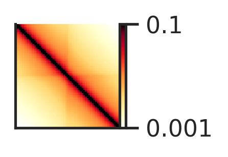
This is the plotting command, which in this case simply takes the path to the file we just produced, the output path, and some arguments to control the esthetics of thefigure.
!plotpup.py --cmap fall --vmax 0.1 --vmin 0.001 \
    --no_score \
    --input_pups local_CTCF_pileup_nonorm.clpy \
    --output local_CTCF_pileup_nonorm.png
INFO:coolpuppy:Can't set both vmin and vmax and get symmetrical scale. Plotting non-symmetrical
INFO:coolpuppy:Saved output to local_CTCF_pileup_nonorm.png
# NBVAL_SKIP
Image('local_CTCF_pileup_nonorm.png')
Pileups by strand
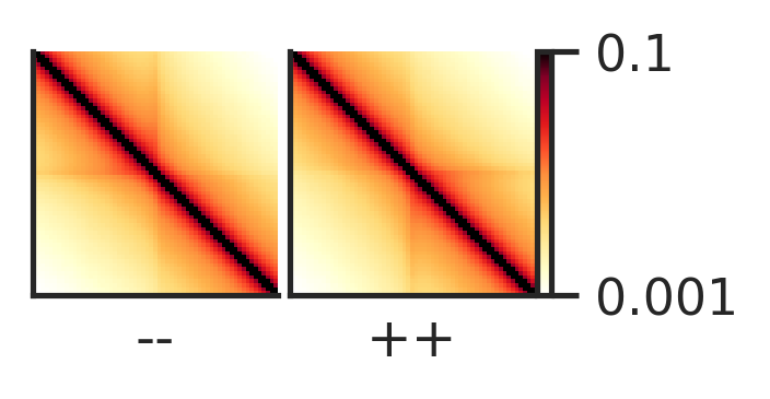
Now let’s split the pileup in two, based on the strands of CTCF sites. There is a simple “preset” for that, you simply need to add --by_strand argument.
!coolpup.py test.mcool::resolutions/10000 test_CTCF.bed.gz \
    --features_format bed --local --nshifts 0 \
    --ignore_diags 0 --view hg38_arms.bed --flank 300000 \
    --by-strand \
    --outname local_CTCF_pileup_bystrand_nonorm.clpy --nproc 2
INFO:coolpuppy:('chr2_p', 'chr2_p'): 1381
INFO:coolpuppy:('chr17_p', 'chr17_p'): 548
INFO:coolpuppy:('chr17_q', 'chr17_q'): 1602
INFO:coolpuppy:Total number of piled up windows: 5752
INFO:coolpuppy:Saved output to local_CTCF_pileup_bystrand_nonorm.clpy
!plotpup.py --cols orientation \
    --col_order "-- ++" \
    --cmap fall --vmax 0.1 --vmin 0.001 \
    --no_score \
    --input_pups local_CTCF_pileup_bystrand_nonorm.clpy \
    --output local_CTCF_pileup_bystrand_nonorm.png
INFO:coolpuppy:Can't set both vmin and vmax and get symmetrical scale. Plotting non-symmetrical
INFO:coolpuppy:Saved output to local_CTCF_pileup_bystrand_nonorm.png
# NBVAL_SKIP
Image('local_CTCF_pileup_bystrand_nonorm.png')
Normalization to background interaction level
Random shifts
Now let’s repeat the above, but also normalize the pileups to the decay of contact probability with separation. You can either use the randomly shifted control regions (here) or a global expected level of interactions calculated for the whole chromosome arm (see below).
!coolpup.py test.mcool::resolutions/10000 test_CTCF.bed.gz \
    --features_format bed --local --by_strand --nshifts 1 \
    --ignore_diags 0 --view hg38_arms.bed --flank 300000 \
    --outname local_CTCF_pileup_bystrand_1shift.clpy --nproc 2
INFO:coolpuppy:('chr2_p', 'chr2_p'): 1381
INFO:coolpuppy:('chr17_p', 'chr17_p'): 548
INFO:coolpuppy:('chr2_q', 'chr2_q'): 2221
INFO:coolpuppy:('chr17_q', 'chr17_q'): 1602
INFO:coolpuppy:Total number of piled up windows: 5752
INFO:coolpuppy:Saved output to local_CTCF_pileup_bystrand_1shift.clpy
!plotpup.py --cols orientation \
    --col_order "-- ++" \
    --no_score \
    --input_pups local_CTCF_pileup_bystrand_1shift.clpy \
    --output local_CTCF_pileup_bystrand_1shift.png
INFO:coolpuppy:Saved output to local_CTCF_pileup_bystrand_1shift.png
# NBVAL_SKIP
Image('local_CTCF_pileup_bystrand_1shift.png')
Chromosome arm-wide expected normalization
While we computed the expected using cooltools python API in the API notebook, here is the CLI version of the same process, with 2 cores.
!cooltools expected-cis --view hg38_arms.bed -p 2 -o test_expected_cis.tsv test.mcool::resolutions/10000
This is a little faster than using random shifts, and in most cases results are very similar. Therefore when a cooler file is used multiple times, it’s beneficial to use this approach.
!coolpup.py test.mcool::resolutions/10000 test_CTCF.bed.gz \
    --features_format bed --local --by_strand --expected test_expected_cis.tsv \
    --ignore_diags 0 --view hg38_arms.bed --flank 300000 \
    --outname local_CTCF_pileup_bystrand_expected.clpy --nproc 2
INFO:coolpuppy:('chr2_p', 'chr2_p'): 1381
INFO:coolpuppy:('chr17_p', 'chr17_p'): 548
INFO:coolpuppy:('chr17_q', 'chr17_q'): 1602
INFO:coolpuppy:Total number of piled up windows: 5752
INFO:coolpuppy:Saved output to local_CTCF_pileup_bystrand_expected.clpy
!plotpup.py --cols orientation \
    --col_order "-- ++" \
    --no_score \
    --input_pups local_CTCF_pileup_bystrand_expected.clpy \
    --output local_CTCF_pileup_bystrand_expected.png
INFO:coolpuppy:Saved output to local_CTCF_pileup_bystrand_expected.png
# NBVAL_SKIP
Image('local_CTCF_pileup_bystrand_expected.png')
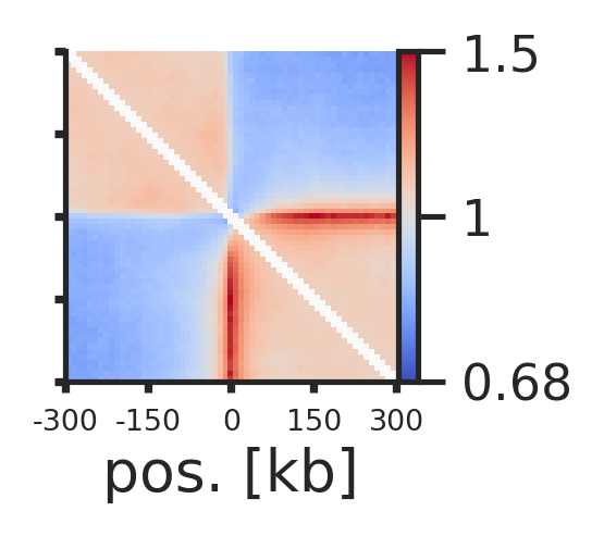
Instead of splitting two strands into two separate pileups, one can also flip the features on the negative strand using --flip_negative_strand. This way a single pileup is created where all features face in the same direction (as if they were on the positive strand). We can also add --plot_ticks to show the central and flanking coordinates on the bottom of the plot.
!coolpup.py test.mcool::resolutions/10000 test_CTCF.bed.gz \
    --features_format bed --local --expected test_expected_cis.tsv \
    --flip_negative_strand --ignore_diags 0 --view hg38_arms.bed --flank 300000 \
    --outname local_CTCF_pileup_flipped_expected.clpy --nproc 2
INFO:coolpuppy:('chr2_p', 'chr2_p'): 1381
INFO:coolpuppy:('chr17_p', 'chr17_p'): 548
INFO:coolpuppy:('chr17_q', 'chr17_q'): 1602
INFO:coolpuppy:Total number of piled up windows: 5752
INFO:coolpuppy:Saved output to local_CTCF_pileup_flipped_expected.clpy
!plotpup.py --plot_ticks --height 1.5 \
    --no_score \
    --input_pups local_CTCF_pileup_flipped_expected.clpy \
    --output local_CTCF_pileup_flipped_expected.png
INFO:coolpuppy:Saved output to local_CTCF_pileup_flipped_expected.png
# NBVAL_SKIP
Image('local_CTCF_pileup_flipped_expected.png')
Arbitrary grouping of snippets for pileups
Now, let’s see if selecting different strength CTCF peaks affects the results. To showcase the power of coolpuppy, we’ll demonstrate how it can be used to generate pileups split be arbitrary categories using groupby. Note that the input peak file needs to include column names in order to use groupby
import pandas as pd
import bioframe
ctcf = bioframe.read_table(ctcf_peaks_file, schema='bed').query(f'chrom in {["chr2", "chr17"]}')
ctcf['quartile_score'] = pd.qcut(ctcf['score'], 4, labels=False) + 1
ctcf.to_csv('ctcf_sites.tsv', sep='\t', index=False, header=True)
!coolpup.py test.mcool::resolutions/10000 ctcf_sites.tsv \
        --features_format bed --local --expected test_expected_cis.tsv \
        --ignore_diags 0 --view hg38_arms.bed --flank 300000 \
        --flip_negative_strand --groupby quartile_score1 \
        --outname groupby_score_CTCF_pileup_expected.clpy --nproc 2
INFO:coolpuppy:('chr2_p', 'chr2_p'): 1381
INFO:coolpuppy:('chr17_p', 'chr17_p'): 548
INFO:coolpuppy:('chr17_q', 'chr17_q'): 1602
INFO:coolpuppy:Total number of piled up windows: 5752
INFO:coolpuppy:Saved output to groupby_score_CTCF_pileup_expected.clpy
!plotpup.py --plot_ticks --height 1.5 \
    --no_score --cols quartile_score1 \
    --col_order '1 2 3 4' \
    --input_pups groupby_score_CTCF_pileup_expected.clpy \
    --output groupby_score_CTCF_pileup_expected.png
INFO:coolpuppy:Saved output to groupby_score_CTCF_pileup_expected.png
# NBVAL_SKIP
Image('groupby_score_CTCF_pileup_expected.png')

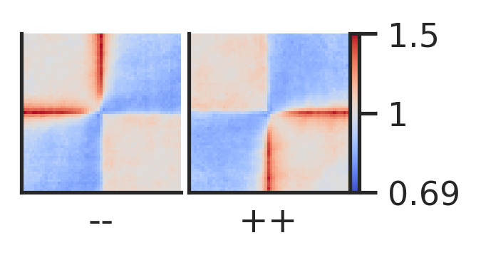
We can also compare interactions between regions (without --local) using the groupby function. However, we need to specify two groups, in this case “quartile_score1” and “quartile_score2”. To limit the number of regions, we use subset with a set seed for reproducibility
!cat ctcf_sites.tsv | awk -F'\t' '($7 > 2)' | \
        coolpup.py test.mcool::resolutions/10000 - \
        --features_format bed --expected test_expected_cis.tsv \
        --view hg38_arms.bed --flank 300000 \
        --mindist 300000 --maxdist 600000 \
        --subset 2000 --seed 1 \
        --groupby quartile_score1 quartile_score2 \
        --outname groupby_CTCF_quartiles_interactions_expected.clpy --nproc 2
INFO:coolpuppy:('chr2_p', 'chr2_p'): 957
INFO:coolpuppy:('chr2_q', 'chr2_q'): 1383
INFO:coolpuppy:('chr17_p', 'chr17_p'): 506
INFO:coolpuppy:('chr17_q', 'chr17_q'): 1963
INFO:coolpuppy:Total number of piled up windows: 4809
INFO:coolpuppy:Saved output to groupby_CTCF_quartiles_interactions_expected.clpy
!plotpup.py --height 0.5 --font_scale 0.5 --vmax 1.5 \
    --no_score --cols quartile_score1 --rows quartile_score2 \
    --col_order '3 4' --row_order '3 4' \
    --input_pups groupby_CTCF_quartiles_interactions_expected.clpy \
    --output groupby_CTCF_quartiles_interactions_expected.png
INFO:coolpuppy:Saved output to groupby_CTCF_quartiles_interactions_expected.png
# NBVAL_SKIP
Image('groupby_CTCF_quartiles_interactions_expected.png')
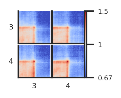
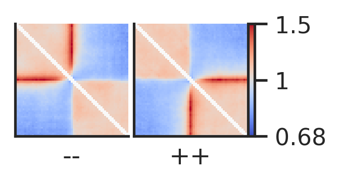
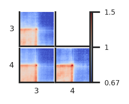
Here we can see all combinations of interactions between quartiles 3 and 4. However, in this case quartile 3-4 and 4-3 interactions are equivalent. To combine them into one (taking into account orientation), we can use the setting --ignore_group_order
!cat ctcf_sites.tsv | awk -F'\t' '($7 > 2)' | \
        coolpup.py test.mcool::resolutions/10000 - \
        --features_format bed --expected test_expected_cis.tsv \
        --view hg38_arms.bed --flank 300000 \
        --mindist 300000 --maxdist 600000 \
        --subset 2000 --seed 1 \
        --groupby quartile_score1 quartile_score2 \
        --ignore_group_order quartile_score \
        --outname groupby_CTCF_quartiles_ignore_order_interactions_expected.clpy --nproc 2
INFO:coolpuppy:('chr2_p', 'chr2_p'): 957
INFO:coolpuppy:('chr2_q', 'chr2_q'): 1383
INFO:coolpuppy:('chr17_p', 'chr17_p'): 506
INFO:coolpuppy:('chr17_q', 'chr17_q'): 1963
INFO:coolpuppy:Total number of piled up windows: 4809
INFO:coolpuppy:Saved output to groupby_CTCF_quartiles_ignore_order_interactions_expected.clpy
!plotpup.py --height 0.5 --font_scale 0.5 --vmax 1.5 \
    --no_score --cols quartile_score1 --rows quartile_score2 \
    --col_order '3 4' --row_order '3 4' \
    --input_pups groupby_CTCF_quartiles_ignore_order_interactions_expected.clpy \
    --output groupby_CTCF_quartiles_ignore_order_interactions_expected.png
INFO:coolpuppy:Saved output to groupby_CTCF_quartiles_ignore_order_interactions_expected.png
# NBVAL_SKIP
Image('groupby_CTCF_quartiles_ignore_order_interactions_expected.png')
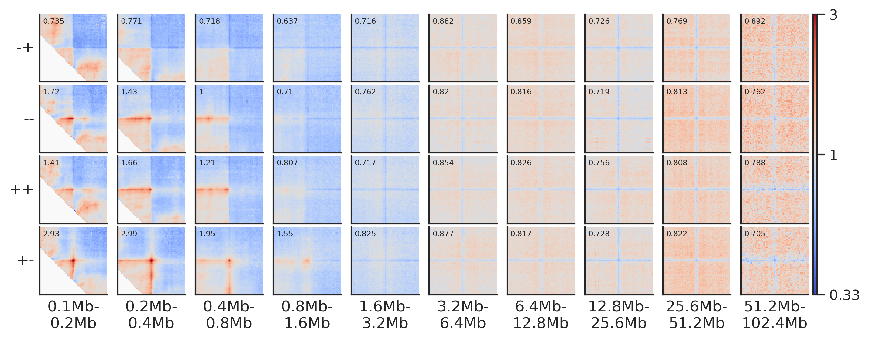
By-distance pileups
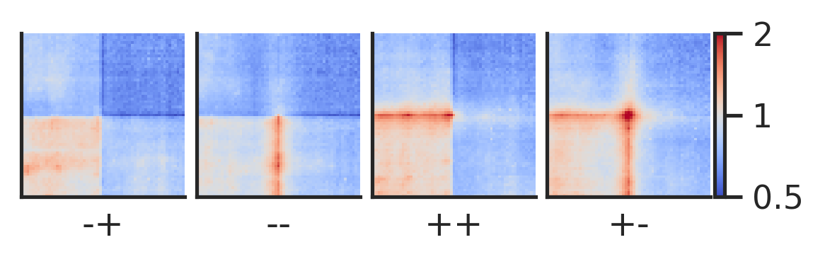
Now we can add another layer of complexity: look at distal interactions betwwen CTCF sites, and split all snippets by their distance.
We use the file that we saved in the python API notebook that contains the annotation of site strength. coolpup.py can accept the coordinate input from stdin, so we can filter that file on the fly using awk, and this way we can use only the strong CTCF sites.
# This command will take a bit longer to run, since it's averaging over a much larger number of snippets
!cat annotated_ctcf_sites.tsv | awk -F'\t' '($11 == "Top by both scores")' | coolpup.py test.mcool::resolutions/10000 - \
    --features_format bed --by_distance --by_strand --expected test_expected_cis.tsv --flip_negative_strand \
    --ignore_diags 0 --view hg38_arms.bed --flank 300000 --mindist 100000 --maxdist 102400000 \
    --outname bydistance_CTCF_pileup_bystrand_expected.clpy --nproc 2
INFO:coolpuppy:('chr2_p', 'chr2_p'): 10250
INFO:coolpuppy:('chr2_q', 'chr2_q'): 15938
INFO:coolpuppy:('chr17_p', 'chr17_p'): 2959
INFO:coolpuppy:('chr17_q', 'chr17_q'): 28284
INFO:coolpuppy:Total number of piled up windows: 57431
INFO:coolpuppy:Saved output to bydistance_CTCF_pileup_bystrand_expected.clpy
# "separation" is created when the pileups are created by distance, and plotpup.py
# always plots them in the order of increasing distance
# We need to specify the order of rows, otherise it's not guaranteed
!plotpup.py --cols separation \
    --rows orientation \
    --row_order "-+ -- ++ +-" \
    --vmax 3 \
    --input_pups bydistance_CTCF_pileup_bystrand_expected.clpy \
    --output bydistance_CTCF_pileup_bystrand_expected.png
INFO:coolpuppy:Saved output to bydistance_CTCF_pileup_bystrand_expected.png
# NBVAL_SKIP
Image('bydistance_CTCF_pileup_bystrand_expected.png')
Now we can also normalize each pileup to the average value in its top-left and bottom-right corners to remove the variation in background level of interactions
!plotpup.py  --cols separation \
    --rows orientation \
    --row_order "-+ -- ++ +-"\
    --vmax 3 --norm_corners 10 \
    --input_pups bydistance_CTCF_pileup_bystrand_expected.clpy \
    --output bydistance_CTCF_pileup_bystrand_expected_corner_norm.png
INFO:coolpuppy:Saved output to bydistance_CTCF_pileup_bystrand_expected_corner_norm.png
# NBVAL_SKIP
Image('bydistance_CTCF_pileup_bystrand_expected_corner_norm.png')

Dividing pileups
Sometimes you may want to compare two pileups directly and plot the result of the division between them. For this we can use the dividepups.py command. Let’s look at all CTCF interactions between 100 kb and 1 Mb by motif orientation.
!cat annotated_ctcf_sites.tsv | awk -F'\t' '($11 == "Top by both scores")' | coolpup.py test.mcool::resolutions/10000 - \
    --features_format bed --by_strand --expected test_expected_cis.tsv \
    --ignore_diags 0 --view hg38_arms.bed --flank 300000 --mindist 100000 --maxdist 1000000 \
    --outname CTCF_pileup_bystrand_expected.clpy --nproc 2
INFO:coolpuppy:('chr2_p', 'chr2_p'): 287
INFO:coolpuppy:('chr2_q', 'chr2_q'): 522
INFO:coolpuppy:('chr17_p', 'chr17_p'): 262
INFO:coolpuppy:('chr17_q', 'chr17_q'): 1235
INFO:coolpuppy:Total number of piled up windows: 2306
INFO:coolpuppy:Saved output to CTCF_pileup_bystrand_expected.clpy
!plotpup.py --cols orientation \
    --col_order "-+ -- ++ +-" \
    --vmax 2 \
    --no_score \
    --input_pups CTCF_pileup_bystrand_expected.clpy \
    --output CTCF_pileup_bystrand_expected.png
INFO:coolpuppy:Saved output to CTCF_pileup_bystrand_expected.png
# NBVAL_SKIP
Image('CTCF_pileup_bystrand_expected.png')
Let’s compare the ++ to the – CTCF motif orientation pileups. First, we have to generate two new pileups for each of the orientations. Importantly, the two pileups cannot differ with regards to the columns they contain and the resolution, flank size etc. they’ve been generated using.
!cat annotated_ctcf_sites.tsv | awk -F'\t' '($11 == "Top by both scores") && ($6 == "+")' | coolpup.py test.mcool::resolutions/10000 - \
    --features_format bed --expected test_expected_cis.tsv \
    --ignore_diags 0 --view hg38_arms.bed --flank 300000 --mindist 100000 --maxdist 1000000 \
    --outname CTCF_pileup_plusstrand_expected.clpy --nproc 2
INFO:coolpuppy:('chr2_p', 'chr2_p'): 78
INFO:coolpuppy:('chr2_q', 'chr2_q'): 122
INFO:coolpuppy:('chr17_p', 'chr17_p'): 67
INFO:coolpuppy:('chr17_q', 'chr17_q'): 293
INFO:coolpuppy:Total number of piled up windows: 560
INFO:coolpuppy:Saved output to CTCF_pileup_plusstrand_expected.clpy
!cat annotated_ctcf_sites.tsv | awk -F'\t' '($11 == "Top by both scores") && ($6 == "-")' | coolpup.py test.mcool::resolutions/10000 - \
    --features_format bed --expected test_expected_cis.tsv \
    --ignore_diags 0 --view hg38_arms.bed --flank 300000 --mindist 100000 --maxdist 1000000 \
    --outname CTCF_pileup_minusstrand_expected.clpy --nproc 2
INFO:coolpuppy:('chr2_p', 'chr2_p'): 62
INFO:coolpuppy:('chr2_q', 'chr2_q'): 118
INFO:coolpuppy:('chr17_p', 'chr17_p'): 53
INFO:coolpuppy:('chr17_q', 'chr17_q'): 324
INFO:coolpuppy:Total number of piled up windows: 557
INFO:coolpuppy:Saved output to CTCF_pileup_minusstrand_expected.clpy
Now we will generate a new pileup of the ratio between the two
!dividepups.py CTCF_pileup_plusstrand_expected.clpy CTCF_pileup_minusstrand_expected.clpy \
    --outname CTCF_pileup_plus_over_minus.clpy
INFO:root:Namespace(input_pups=['CTCF_pileup_plusstrand_expected.clpy', 'CTCF_pileup_minusstrand_expected.clpy'], outname='CTCF_pileup_plus_over_minus.clpy')
INFO:root:Saved output to CTCF_pileup_plus_over_minus.clpy
!plotpup.py --no_score --cmap PuOr_r \
    --input_pups CTCF_pileup_plus_over_minus.clpy \
    --output CTCF_pileup_plus_over_minus.png
INFO:coolpuppy:Saved output to CTCF_pileup_plus_over_minus.png
# NBVAL_SKIP
Image('CTCF_pileup_plus_over_minus.png')
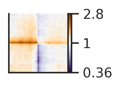
If you want to quickly plot the division of two pileups without saving the intermediate, this can also be done directly in plotpup.py with the argument --divide_pups
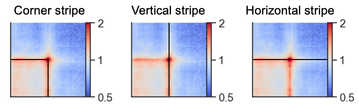
Stripe stackups
Oftentimes, as seen in the examples above, the interactions between regions are not just focal, but seen as stripes with enrichment along the vertical/horizontal axis from one or both of the anchor points. In the CTCF pileups from above we see a very strong corner stripe between +- sites, so let’s try to plot these individual stripes. Below is a schematic of what is meant by the different types of stripes.
!cat annotated_ctcf_sites.tsv | awk -F'\t' '($11 == "Top by both scores")' | coolpup.py test.mcool::resolutions/10000 - \
    --features_format bed --by_strand --expected test_expected_cis.tsv \
    --ignore_diags 0 --view hg38_arms.bed --flank 300000 --mindist 100000 --maxdist 1000000 \
    --outname bystrand_CTCF_pileup_bystrand_expected_stripes.clpy --nproc 2 --store_stripes
INFO:coolpuppy:('chr2_p', 'chr2_p'): 287
INFO:coolpuppy:('chr2_q', 'chr2_q'): 522
INFO:coolpuppy:('chr17_p', 'chr17_p'): 262
INFO:coolpuppy:('chr17_q', 'chr17_q'): 1235
INFO:coolpuppy:Total number of piled up windows: 2306
INFO:coolpuppy:Saved output to bystrand_CTCF_pileup_bystrand_expected_stripes.clpy
In the pileups we see a very strong corner stripe between +- sites, so let’s try to plot these individual stripes using the --stripe argument. Below is a schematic of what is meant by the different types of stripes.
!plotpup.py --rows orientation  \
    --row_order "+-" --stripe corner_stripe \
    --vmax 10 --height 1.5 --font_scale 0.75 --plot_ticks \
    --input_pups bystrand_CTCF_pileup_bystrand_expected_stripes.clpy \
    --output bystrand_CTCF_pileup_+-_expected_cornerstripe.png
INFO:coolpuppy:Saved output to bystrand_CTCF_pileup_+-_expected_cornerstripe.png
# NBVAL_SKIP
Image('bystrand_CTCF_pileup_+-_expected_cornerstripe.png')
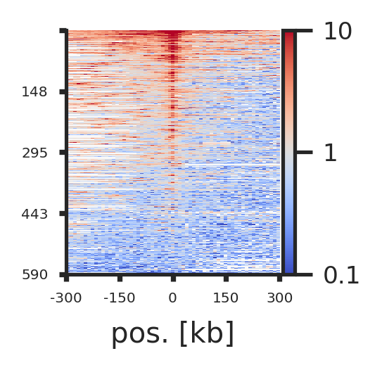
Each line of the above plot represents the “corner stripe” between two regions. These pairs are sorted by the sum of the stripe by default, but we can also sort them by the central pixel, i.e. the pixel where the two regions of interest interact, with the --stripe_sort argument. We can further save the pairs in the sorted order using --out_sorted_bedpe. This file can then be used to inspect individual pairs with high contact frequencies. We can also add a lineplot with the average signal above the stripes using --lineplot (note that this only works for single stripe plots.)
!plotpup.py --rows orientation  \
    --row_order "+-" --stripe corner_stripe \
    --vmax 10 --height 1.5 --font_scale 0.75 --plot_ticks \
    --input_pups bystrand_CTCF_pileup_bystrand_expected_stripes.clpy \
    --output bystrand_CTCF_pileup_+-_expected_cornerstripe_centersort.png \
    --stripe_sort center_pixel --out_sorted_bedpe CTCF_+-_sorted_centerpixel.bedpe \
    --lineplot
INFO:coolpuppy:Saved output to bystrand_CTCF_pileup_+-_expected_cornerstripe_centersort.png
# NBVAL_SKIP
Image('bystrand_CTCF_pileup_+-_expected_cornerstripe_centersort.png')

Rescaling
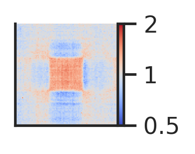
Pileups can also be rescaled to visualise enrichment within regions of interests of different sizes using --rescale. The --rescale_flank value represents how large the flanks are compared to the region of interest, where 1 is equal in size and for example 3 will be a three times the size. The number of pixels in the final plot after rescaling is set with --rescale_size. Let’s try this for A compartment interactions.
!coolpup.py test.mcool::resolutions/10000 A_compartments.bed \
    --features_format bed --expected test_expected_hg38_cis.tsv \
    --ignore_diags 0 \
    --rescale --rescale_flank 1 --rescale_size 99 \
    --outname A_compartment_pileup_rescaled_expected.clpy --nproc 2
INFO:coolpuppy:Rescaling with rescale_flank = 1.0 to 99x99 pixels
INFO:coolpuppy:('chr17', 'chr17'): 253
INFO:coolpuppy:Total number of piled up windows: 1528
INFO:coolpuppy:Saved output to A_compartment_pileup_rescaled_expected.clpy
!plotpup.py --vmax 2 --no_score \
    --input_pups A_compartment_pileup_rescaled_expected.clpy \
    --output A_compartment_pileup_rescaled_expected.png
INFO:coolpuppy:Saved output to A_compartment_pileup_rescaled_expected.png
# NBVAL_SKIP
Image('A_compartment_pileup_rescaled_expected.png')
Trans (inter-chromosomal) pileups
We can also perform pileups between regions on different chromosomes. We will try this for A-A compartments again. To perform the same analysis between chromosomes, we need to use an expected file for trans (or use shifted controls) and then run the analysis with --trans.
!coolpup.py test.mcool::resolutions/10000 A_compartments.bed \
    --features_format bed --expected test_expected_trans.tsv \
    --trans \
    --rescale --rescale_flank 1 --rescale_size 99 \
    --outname A_compartment_pileup_rescaled_trans_expected.clpy
/gpfs/igmmfs01/eddie/wendy-lab/elias/coolpuppy_stable/coolpuppy/coolpuppy/coolpup.py:2156: UserWarning: Ignoring maxdist when using trans
  CC = CoordCreator(
INFO:coolpuppy:Rescaling with rescale_flank = 1.0 to 99x99 pixels
INFO:coolpuppy:('chr2', 'chr17'): 1173
INFO:coolpuppy:Total number of piled up windows: 1173
INFO:coolpuppy:Saved output to A_compartment_pileup_rescaled_trans_expected.clpy
!plotpup.py --vmax 2 --no_score \
    --input_pups A_compartment_pileup_rescaled_trans_expected.clpy \
    --output A_compartment_pileup_rescaled_trans_expected.png
INFO:coolpuppy:Saved output to A_compartment_pileup_rescaled_trans_expected.png
# NBVAL_SKIP
Image('A_compartment_pileup_rescaled_trans_expected.png')
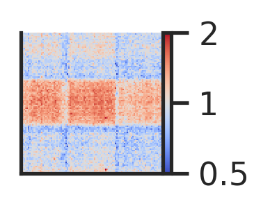
Here we can see rescaled A-A interactions across chromosomes. The pileups look less good than in cis due to the sparse data used in this example.